
In brief
- Every reliability distribution is the same object described four different ways, and each of the four functions can be derived from any one of the rest.
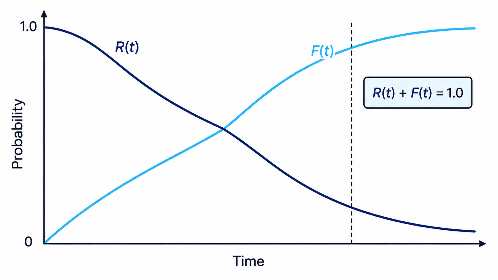
- F(t) is the probability an item has failed by time t and R(t) is its complement, so the two account for the whole population between them.
- f(t) is unconditional and always measures failures against the full population that started the clock, while h(t) measures them against the population that has actually survived to time t.
- The master relationship says the entire survival history of a population is fully determined by its hazard rate history and nothing else.
- The shape of h(t) is what decides whether a time-based maintenance task has anything to act on, because a scheduled replacement can only reduce risk against a hazard rate that is genuinely rising with age.
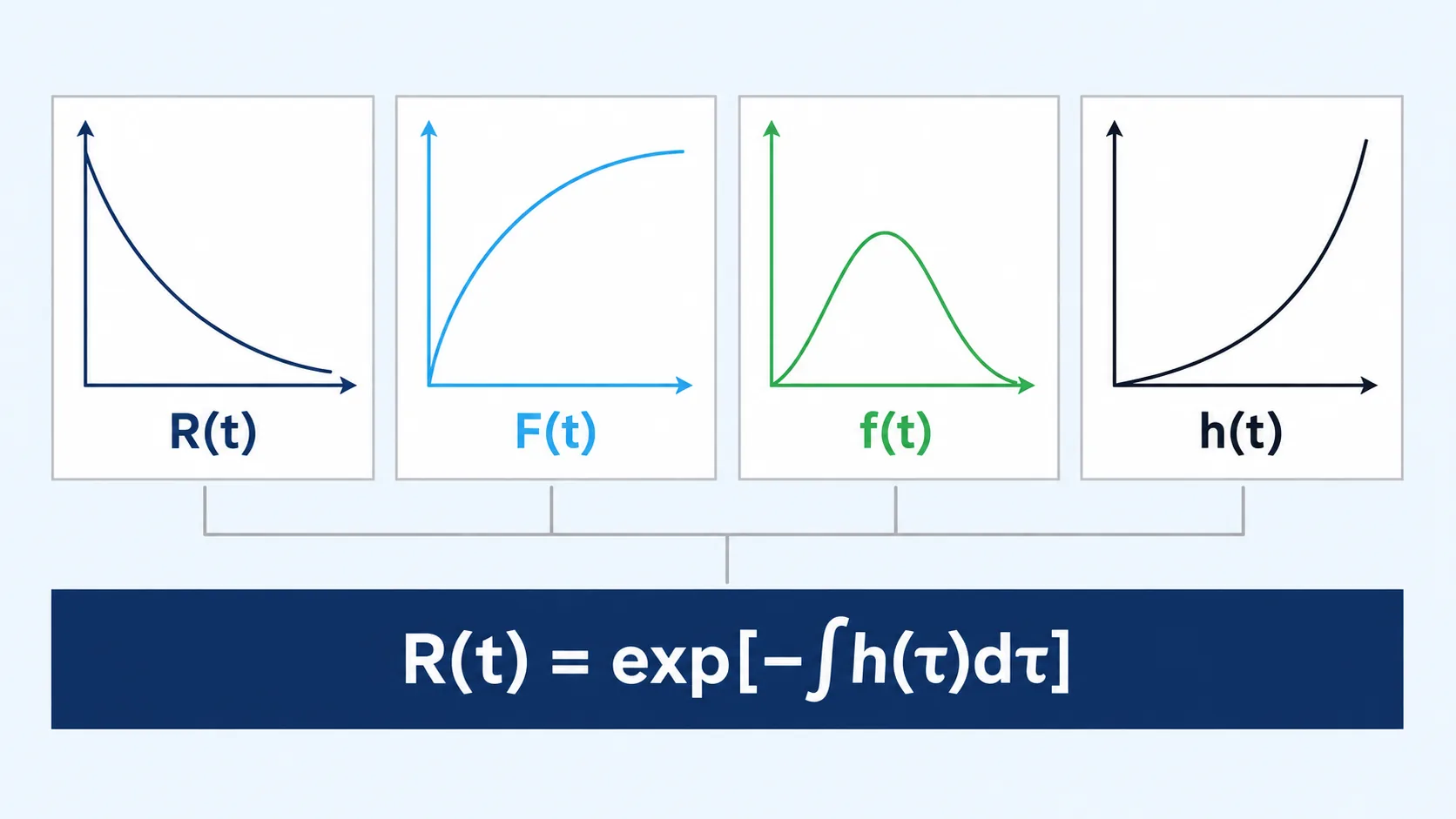
Every reliability distribution you will ever fit, plot or defend is the same object described four different ways. Once that stops being an abstract claim and becomes something you can see in a set of numbers, the rest of the discipline reorganises itself. A Weibull, a lognormal, an exponential: each one is simply a different assumed shape for a single function, and everything else follows from it by calculus alone.
That function is the hazard rate, h(t), and it is the engineering-useful member of the family because it is conditional on survival. It does not ask what fraction of a population fails at time t. It asks: given that this item has already made it to time t, what is its risk right now? That is the question a maintenance planner is actually asking when they schedule an inspection, and it is the question none of the other three functions can answer directly.
This page builds all four functions from first principles, shows exactly how each one is derived from the others, and carries one original data set through all four so the connections stop being symbolic and start being numbers you could reproduce yourself. By the end, R(t) = exp[−∫h(τ)dτ] should read as an obvious consequence rather than a formula to memorise, because that single relationship is the mathematical spine the rest of this series is built on.
Four Functions, One Failure Behaviour
Start with a population of identical items placed into service at time zero and run until every one of them has failed.
Each item has a time to failure, and across the population those times form a distribution. Four functions describe that same distribution from four different angles, and none of them is more fundamental than the others; each can be derived from any one of the rest.
F(t), the cumulative distribution function, is the probability that an item has failed by time t. R(t), the reliability function, is its complement: the probability of surviving beyond t (MIL-HDBK-338B 1998). Because an item has either failed or survived by any given time, the two account for the whole population between them.
- R(t)
- the reliability function, the probability of surviving beyond time t
- F(t)
- the cumulative distribution function, the probability of having failed by time t
f(t), the probability density function, is the rate at which the original population fails at time t, expressed as a fraction of that original population per unit of time. It is the slope of F(t), and equivalently the negative slope of R(t) (MIL-HDBK-338B 1998).
- f(t)
- the probability density function, the instantaneous failure rate per unit of the original population
f(t) is unconditional. It always measures failures against the full population that started the clock, never against however many items are still running at time t. That distinction is easy to state and easy to lose sight of, and the worked example later on this page makes it concrete with numbers.
The Hazard Rate: Conditioning on Survival Changes the Question
h(t), the hazard rate, asks a narrower and more useful question. Instead of measuring failures against the original population, it measures them against the population that has actually survived to time t.
- h(t)
- the hazard rate, the instantaneous rate of failure at time t, conditional on survival to t
- f(t)
- the probability density function at time t
- R(t)
- the probability of having survived to time t
Dividing the unconditional failure density f(t) by the surviving fraction R(t) rescales the failure rate onto the population that is actually still exposed to risk at that moment. As t increases, R(t) shrinks, so the same absolute rate of failure gets divided by a smaller and smaller surviving group. That is precisely why h(t) can keep climbing even after f(t) has started to fall: fewer items are failing in absolute terms, but they are a growing share of an ever-thinner surviving population (MIL-HDBK-338B 1998).
This is the function a maintenance decision actually needs, because a maintenance decision is never made about the original population. It is made about the specific unit in front of you right now, which has already proven it can survive to its current age. h(t) answers that question directly; f(t) cannot.
The Master Relationship: R(t) = exp[−∫h(τ)dτ]
The hazard rate can also be built up the other way, from h(t) back to R(t), and the route there is short enough to walk through in full.
Step 1. Start from the definition of the hazard rate. h(t) = f(t)/R(t), and f(t) = −dR(t)/dt, so:
The reason for taking this step is that it turns the hazard rate into a differential equation in R(t) alone, which can be solved directly.
Step 2. Recognise the right-hand side as a derivative of a logarithm. The expression −[dR/dt]/R is exactly −d[ln R(t)]/dt, so:
This step matters because it converts a ratio into a clean derivative, which is what makes the next step possible by straightforward integration.
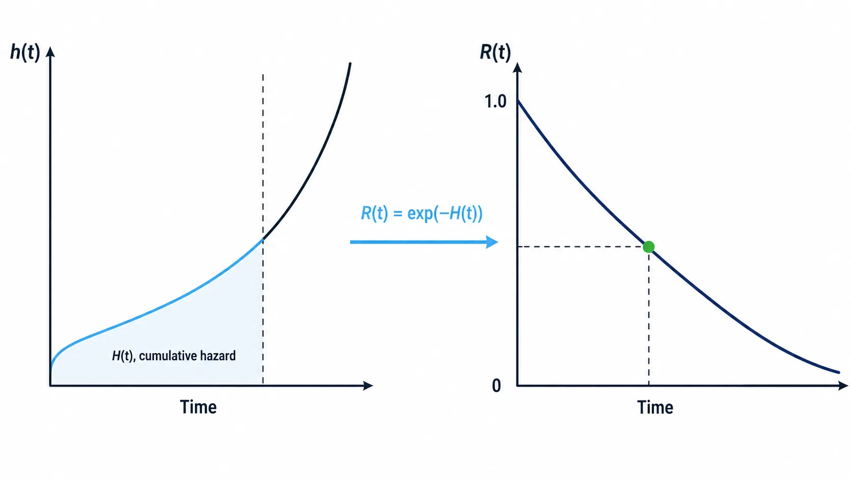
Step 3. Integrate both sides from 0 to t. Since R(0) = 1 for any population that starts fully intact, ln R(0) = 0, and integrating gives:
The reason for integrating is that h(t) is a rate, and accumulating a rate over an interval is exactly what an integral does; this accumulated quantity has its own name, the cumulative hazard.
Step 4. Exponentiate to solve for R(t).
- R(t)
- the reliability function at time t
- h(τ)
- the hazard rate at each instant τ between 0 and t
- ∫₀ᵗ h(τ) dτ
- the cumulative hazard, the running total of instantaneous risk accumulated from time 0 to time t
This is the master relationship of the whole discipline (MIL-HDBK-338B 1998). It says that the entire survival history of a population is fully determined by its hazard rate history, and nothing else. Every named distribution in reliability engineering, Weibull, exponential, lognormal, is simply a different assumed shape for h(t), pushed through this one equation. Learn to read h(t) and you can read every distribution built on it.
The accumulated quantity inside the exponent is useful enough to name on its own. Call it H(t), the cumulative hazard function.
- H(t)
- the cumulative hazard function, the total accumulated risk from time 0 to time t
H(t) has no upper bound and is not itself a probability; it is the running total that the exponential function converts into one. As H(t) climbs from 0 toward infinity, e to the power minus H of t falls from 1 toward zero, which is exactly the behaviour a reliability function must have.
One Population, Four Descriptions: A Worked Example
Take a fleet of 1,000 identical conveyor drive gearbox output bearings, all commissioned at the same time and run under the same duty. Their time to failure follows a Weibull hazard with shape parameter β = 3.2 and scale parameter η = 20,000 operating hours, a shape consistent with a cumulative fatigue mechanism in the bearing races. (The Weibull form itself is the subject of a later page in this series; here it is only the source of the numbers, and every figure below was computed and independently verified before this page was drafted.)
The table below reads the same population through all four functions at five points on the operating-hour clock.
| t (operating hours) | R(t) | F(t) | f(t) | h(t) |
|---|---|---|---|---|
| 5,000 | 0.9882 | 0.0118 | 0.0000075 | 0.0000076 |
| 10,000 | 0.8969 | 0.1031 | 0.0000312 | 0.0000348 |
| 15,000 | 0.6715 | 0.3285 | 0.0000571 | 0.0000850 |
| 20,000 | 0.3679 | 0.6321 | 0.0000589 | 0.0001600 |
| 25,000 | 0.1297 | 0.8703 | 0.0000339 | 0.0002614 |
Two things are worth reading directly off this table. R(t) and F(t) sum to 1.0000 at every row, exactly as the complement relationship requires. And f(t) rises then falls, peaking somewhere around 20,000 hours, while h(t) simply keeps climbing across the whole range. That difference in shape is the conditioning at work, and it is worth making concrete rather than leaving it as a curve on a chart.
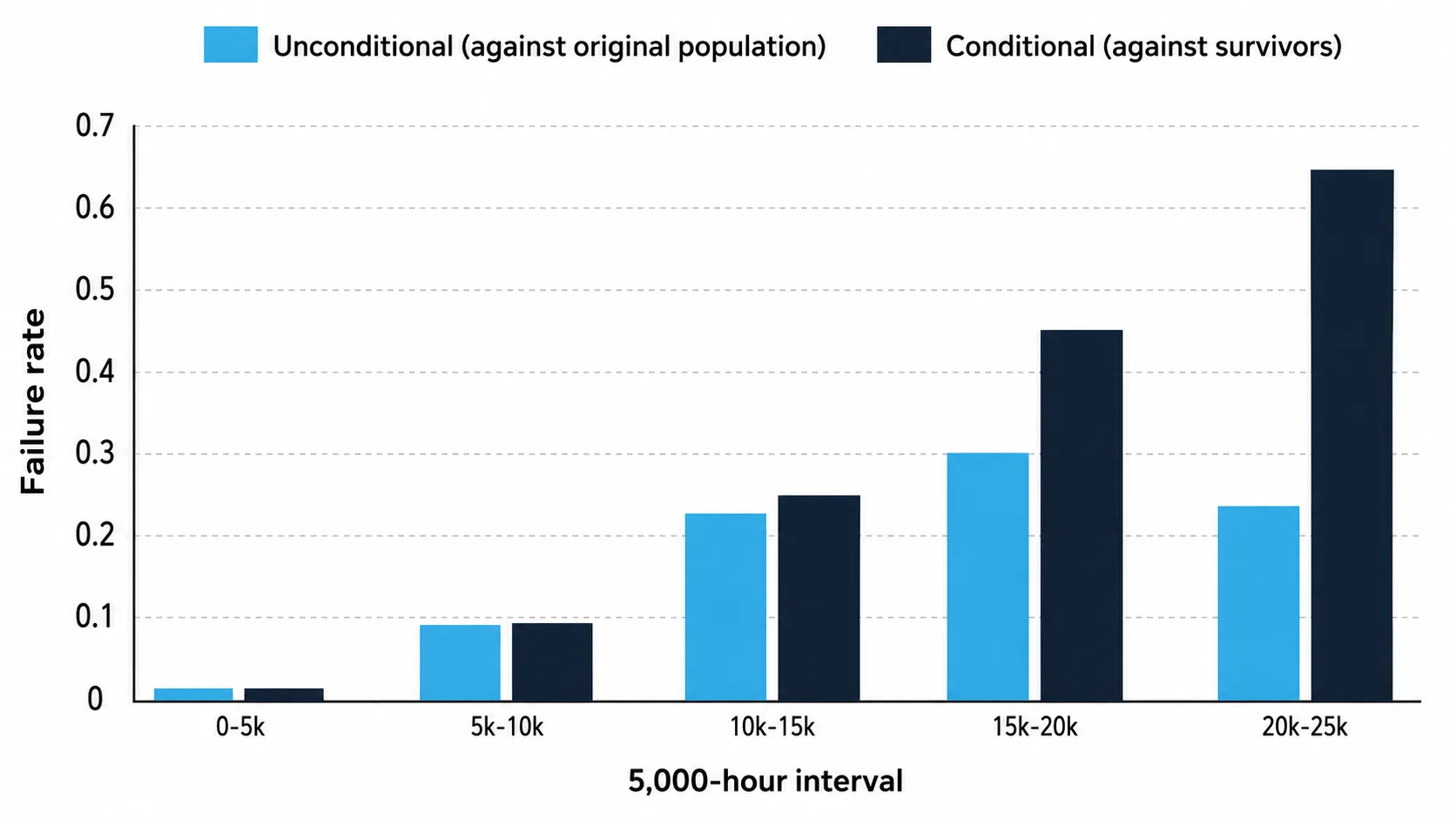
Convert the same distribution into whole bearings out of the original 1,000, counted in 5,000-hour bands:
| Interval (hours) | Survivors at start | New failures in interval | Unconditional rate (against the original 1,000) | Conditional rate (against survivors at start) |
|---|---|---|---|---|
| 0 to 5,000 | 1,000 | 12 | 0.012 | 0.012 |
| 5,000 to 10,000 | 988 | 91 | 0.091 | 0.092 |
| 10,000 to 15,000 | 897 | 226 | 0.226 | 0.252 |
| 15,000 to 20,000 | 671 | 303 | 0.303 | 0.452 |
| 20,000 to 25,000 | 368 | 238 | 0.238 | 0.647 |
Read the last row carefully, because it is where the two framings diverge the most. Against the original 1,000 bearings, only 23.8% fail in that final band, a figure lower than the band before it, and a naive read of that number alone would suggest risk is easing. But of the 368 bearings that actually made it to 20,000 hours, 64.7% of them fail before 25,000. Both numbers are correct. They are answers to different questions. The unconditional column is what f(t) is measuring; the conditional column is what h(t) is measuring, and it is the one that tells a bearing still running at 20,000 hours what its actual risk looks like from where it stands. This is the distinction most readers miss on first exposure to hazard rate, and it is the reason h(t) earns the central place in this series.
The Constant-Hazard Special Case
One shape of h(t) is common enough, and simple enough, to be worth naming on its own: a hazard rate that does not change with age at all.
- λ
- a constant hazard rate, independent of age
This follows directly from the master relationship: integrating a constant λ from 0 to t gives H of t equals lambda t, and R of t equals e to the power minus H of t becomes e to the power minus lambda t. It is the exponential distribution, and it carries a property that makes it mathematically convenient and physically restrictive at the same time: an item with a constant hazard rate is, in a precise sense, no more and no less likely to fail in the next hour regardless of how many hours it has already run. Age carries no information.
That property is exactly why the constant-hazard case should be treated as a special case rather than a default assumption. Most physical degradation mechanisms, fatigue, wear, corrosion, do carry information in age, which means their hazard rate is not constant. Reaching for e to the power minus lambda t because it is the simplest formula to hand, rather than because the mechanism has been shown to be memoryless, is one of the more consequential shortcuts in applied reliability work, because every conclusion drawn from it inherits the assumption silently.
What Shapes Can the Hazard Rate Take?
The master relationship works for any shape of h(t) at all, which raises the obvious next question: what shapes actually occur, and what do they mean physically?
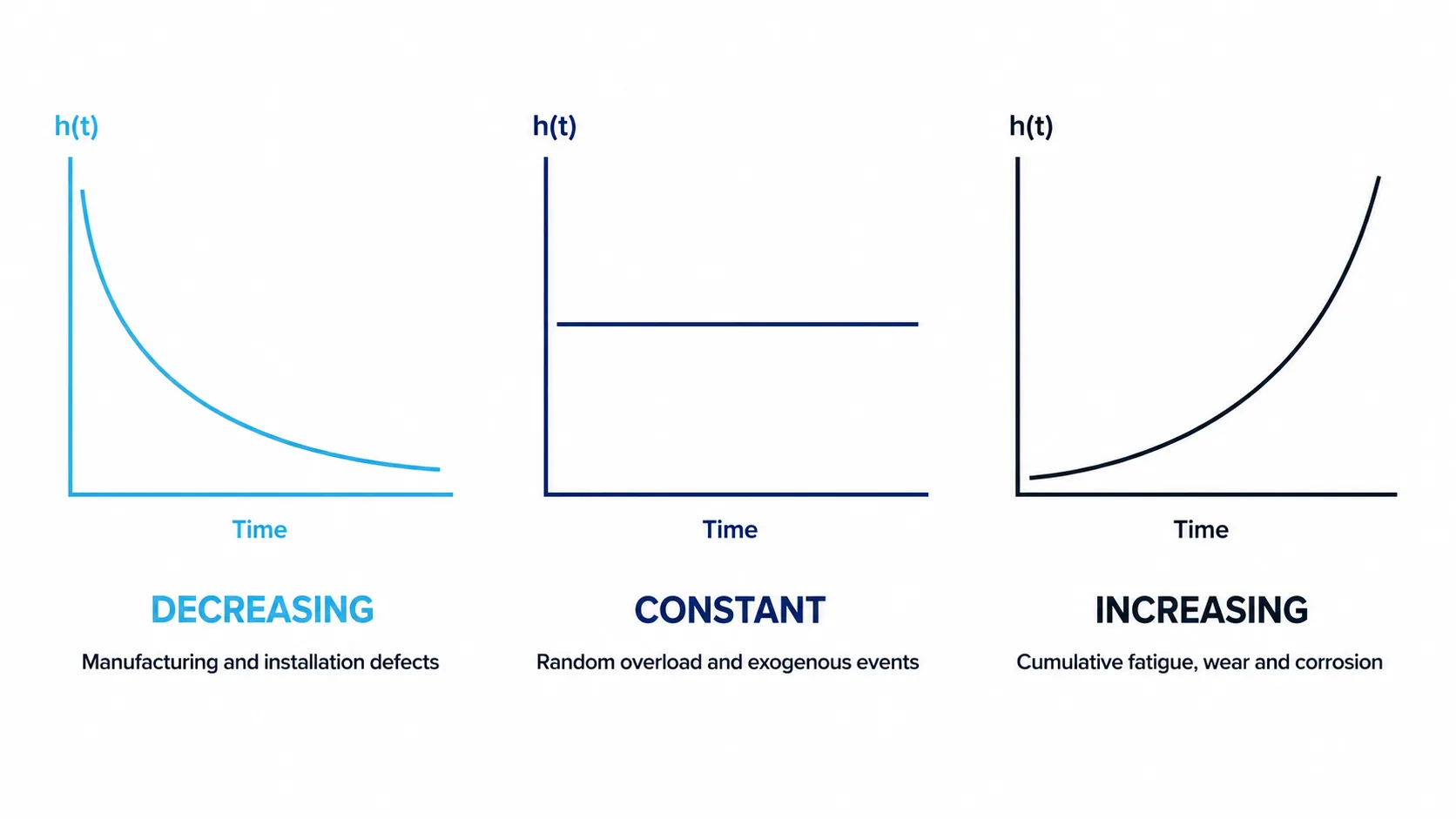
Three shapes cover the physical cases a reliability engineer meets in practice, and each has a distinct mechanism behind it (Abernethy 2006).
A decreasing hazard rate falls with age. Physically, this is the signature of manufacturing, installation and commissioning defects: a weak weld, a contaminated lubricant charge, an incorrectly torqued fastener. Items with these defects tend to fail early, and once they have failed and left the population, the survivors are, on average, the better-built units, so the remaining risk falls.
A constant hazard rate, covered above, is the signature of failure driven by random overload or exogenous events unrelated to age: a lightning-induced power surge, a foreign object ingested into a process stream, an operator error. These events are no more likely on an old item than a new one.
An increasing hazard rate rises with age, the signature of cumulative damage: fatigue, wear, corrosion, insulation ageing. The bearing example above is exactly this case, built with β = 3.2, and the last row of the interval table is the increasing hazard made visible in whole numbers.
The shape is the whole point, and it is worth stating why directly: the shape of h(t), not the mere existence of a calendar age, decides whether a time-based maintenance task has anything to act on. A time-based replacement can only reduce risk against a hazard rate that is genuinely rising with age. Against a decreasing or constant hazard rate, replacing an item on a fixed schedule does not reduce risk and can introduce new risk, because the replacement itself is a fresh, unproven item entering the decreasing-hazard region. This series returns to the mathematics behind selecting β from data later on (see the Weibull page ahead in this series), and to the decision consequence of an increasing hazard rate near the end.
One further piece of vocabulary is worth being precise about here, because it prevents a genuinely common mix-up. h(t) applies to a non-repairable item's time to its one, single failure. A repairable system, one that is fixed and returned to service rather than discarded, accumulates a stream of failure events over its life, and the correct description of that stream is the rate of occurrence of failures, or ROCOF, not a hazard rate. A constant failure rate λ is a special case that can describe either situation, which is exactly why it gets treated as a general property when it is not one (MIL-HDBK-338B 1998). Keeping hazard rate, failure rate and ROCOF as three distinct terms, rather than three names for the same idea, is what lets the rest of this series gate correctly on whether an item is analysed with a life distribution or with an event-process method, a distinction the next page in this series turns into a hard rule.
Reading the Four Functions Together
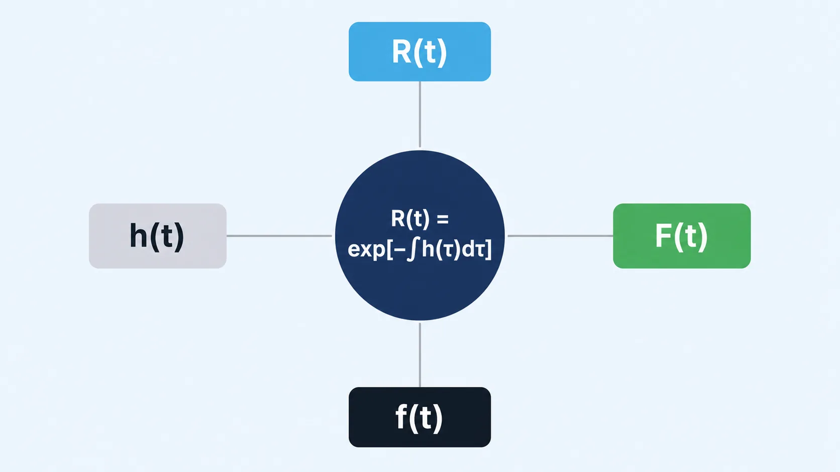
Four functions, one distribution, and a single equation joining them all: R(t) = exp[−∫h(τ)dτ]. F(t) and R(t) tell you where the population stands at time t. f(t) tells you the unconditional rate at which the original population is failing. h(t) tells you the conditional rate, the one a maintenance decision actually needs, because it answers the question the item in front of you is actually asking: given that I have survived this far, what is my risk now?
Every technique later in this series is a way of estimating, shaping or acting on h(t). A Weibull fit estimates its shape from data. A probability plot displays that estimate. A reliability block diagram composes component-level R(t) into a system-level R(t). A replacement interval calculation reads the shape of h(t) and decides whether a scheduled task has anything to act on. None of it requires new mathematics beyond what is on this page; it requires applying the same four functions and the same master relationship to progressively more realistic data and more realistic systems.
Frequently asked questions
What is the hazard rate h(t) in reliability engineering?
The hazard rate h(t) is the instantaneous rate of failure at time t, conditional on survival to t, and it is calculated as h(t) = f(t) / R(t). Instead of measuring failures against the original population, it measures them against the population that has actually survived to time t. That is the function a maintenance decision actually needs, because a maintenance decision is never made about the original population: it is made about the specific unit in front of you, which has already proven it can survive to its current age.
What is the difference between the probability density function and the hazard rate?
f(t) is unconditional. It always measures failures against the full population that started the clock, never against however many items are still running at time t. h(t) divides that same failure density by the surviving fraction R(t), which rescales it onto the population still exposed to risk. As t increases R(t) shrinks, so h(t) can keep climbing even after f(t) has started to fall. In the worked example on this page, 23.8% of the original 1,000 bearings fail in the final band while 64.7% of the 368 that reached 20,000 hours fail before 25,000. Both numbers are correct; they answer different questions.
What is the master relationship between the reliability functions?
R(t) equals the exponential of minus the integral of h(tau) d tau from 0 to t. It says that the entire survival history of a population is fully determined by its hazard rate history, and nothing else. Every named distribution in reliability engineering, Weibull, exponential and lognormal among them, is simply a different assumed shape for h(t) pushed through this one equation, which is why learning to read h(t) lets you read every distribution built on it.
What shapes can the hazard rate take, and what do they mean?
Three shapes cover the physical cases met in practice. A decreasing hazard rate is the signature of manufacturing, installation and commissioning defects: those items fail early and, once they leave the population, the survivors are on average the better-built units. A constant hazard rate is the signature of failure driven by random overload or exogenous events unrelated to age. An increasing hazard rate is the signature of cumulative damage: fatigue, wear, corrosion and insulation ageing. The shape matters because a time-based replacement can only reduce risk against a hazard rate that is genuinely rising with age.