
In brief
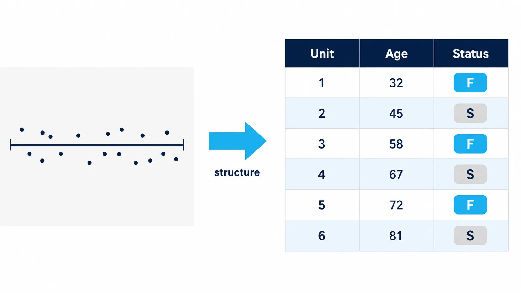
- A life data set is a list of ages, each belonging to a single unit, each labelled with what happened to that unit at that age: it either failed by the target failure mode, or it did not.
- The time base is the exposure measure the age clock runs on, and calendar time, the number of days since commissioning, almost never is the right one.
- There are four recognised kinds of censoring, and truncation is a different problem again: censoring means incomplete information about a unit in the data set, truncation means the unit never entered it.
- Suspensions carry real survival information, so dropping them understates the population at risk and pushes the fitted distribution toward an earlier apparent failure age.
- One question gates everything: is this a sample of lifetimes from a population of comparable items, or a sequence of events on one continuously operating system?
Every Weibull plot, every characteristic life, every replacement interval later in this series rests on one thing nobody teaches with much care: the life data set underneath it. Get the data structure wrong and the analysis that follows is confident, defensible-looking and invalid. Get it right and the rest of the discipline follows cleanly from what is actually a small set of rules.
Most of what separates a usable life data set from an unusable one happens before any curve is fitted: choosing the right clock, classifying every observation correctly, and knowing which units belong in the analysis at all. None of it is difficult once stated plainly, and all of it is easy to get wrong quietly, in a spreadsheet, without anything obviously breaking.
This page covers what a life data set actually is, how to choose its time base, the ways an observation can be incomplete, why the incomplete ones still carry information, and the one gate every data set must pass before a distribution is fitted to it at all.
What a Life Data Set Actually Is
A life data set is a list of ages, each belonging to a single unit, each labelled with what happened to that unit at that age: it either failed by the target failure mode, or it did not.
Every row needs the age itself, on a declared and consistent time base, and a status. Nothing more is strictly required to begin an analysis, though a well-run CMMS extraction, covered later on this page, captures more than this minimum.
- t_i
- the age of unit i, recorded on the declared time base, at the point it was last observed
- delta_i
- the status of unit i at that age: F for a genuine failure of the target mode, S for a suspension
- N
- n_F + n_S, the total record count, failures plus suspensions
Two disciplines make this structure defensible rather than decorative. Every age must sit on the same time base; mixing hours for some units and calendar days for others invalidates the set before any statistics touch it. And every failure must be the same failure mode. A data set that mixes a bearing's fatigue failures with the same bearing's lubrication failures is not one life distribution, it is two, and forcing a single fit through mixed modes produces a plot that looks plausible and explains nothing.
Choosing the Time Base: Why Calendar Time Is Usually Wrong
The time base is the exposure measure the age clock runs on, and it deserves a deliberate decision rather than a default. Operating hours, load cycles, start counts, tonnes processed and kilometres are all legitimate time bases. Calendar time, the number of days since commissioning, almost never is.
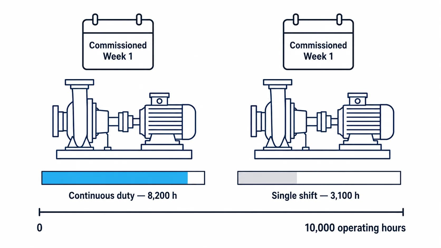
The reason is straightforward. Two identical pumps commissioned the same week can accumulate very different exposure if one runs a single shift and the other runs continuously, and a fatigue mechanism responds to accumulated cycles or hours, not to the calendar. Fitting a distribution to calendar age when the mechanism is duty-driven mixes units with genuinely different risk into the same nominal age, and the resulting β and η describe neither unit correctly.
Choosing it is a short, disciplined argument, not a lookup:
- Identify the degradation mechanism. Fatigue accumulates with load cycles or running hours; wear accumulates with throughput or distance; a starter motor's ring gear wears with start events, not running hours. The mechanism decides the exposure measure it responds to.
- Confirm the measure is consistently recorded. A time base that exists in engineering theory but not in the CMMS or control system historian is not usable yet; the extraction work later on this page has to close that gap first.
- Check the measure varies meaningfully across the fleet. Where duty is near-identical, calendar time and operating hours track closely enough that the choice matters less; where duty varies, as it usually does, only the mechanism-driven measure produces a defensible fit.
A crusher liner wears against tonnes processed, a standby generator's starter system against start counts rather than hours run. A slurry pump mechanical seal, the case this page carries through its main worked example, wears against operating hours, because seal face wear accumulates with running time under load.
The Four Kinds of Censoring, and How Truncation Differs
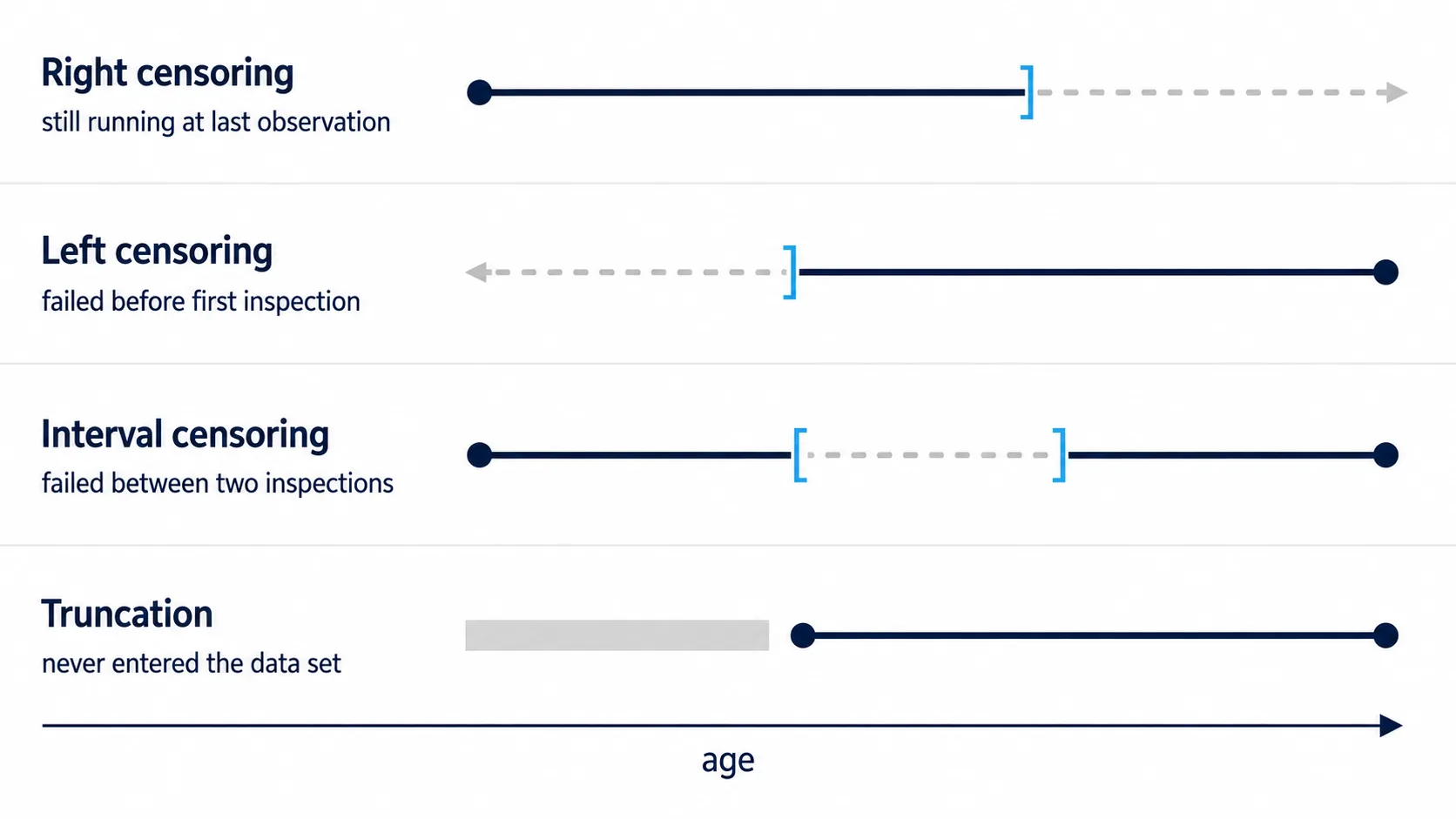
Not every unit in a life data set gives you its exact failure age. An observation is censored when the unit is genuinely part of the data set but its failure time is only partly known. There are four recognised kinds.
Right censoring, also called a suspension, is the most common in operational data. The unit has not failed by the target mode at its last observed age: it might still be running, it might have been removed intact for an unrelated reason, or it might still be in service when the data set was cut off. A mechanical seal removed from a pump for an unrelated impeller change, its face still serviceable, is a right-censored observation.
Left censoring occurs when a unit is known to have failed before a certain age, but the exact age is unknown. An idler bearing found seized at the first scheduled inspection after installation has failed left-censored: the failure happened sometime between commissioning and that inspection, and nothing narrower is known.
Interval censoring occurs when the failure is known to lie between two inspection points. A mill liner segment found worn beyond its rejection limit at a 2,000-hour inspection, but confirmed intact at the previous 1,500-hour inspection, failed somewhere in that 500-hour window. This is the natural consequence of periodic inspection rather than continuous monitoring.
Truncation is a different problem, and worth distinguishing clearly because it is often confused with censoring. Censoring means a unit is in the data set with incomplete information about its failure time. Truncation means the sampling process never lets certain units into the data set at all. A CMMS that only retains work order history for the last three years will simply never show a unit that failed and left service before that window began. That unit is not censored, it is truncated out of the sample, and treating a truncated data set as though it were only right-censored understates how much early failure history has actually gone missing.
Suspensions Carry Information: Why Dropping Them Biases the Result
Suspensions are never plotted as points, because they carry no known failure age to plot. That fact leads to a natural but costly mistake: treating suspensions as though they can simply be removed from the data set. They cannot. A suspension tells you the unit survived to at least its recorded age, and that is real survival information, not an absence of information (Abernethy 2006).
The mechanism is direct. Dropping suspensions and analysing only the failures as if they were a complete sample understates the population actually at risk, and it silently converts each failure into a larger fraction of that smaller, wrong population. Every failure looks like it represents more of the fleet than it actually does, which pushes the fitted distribution toward an earlier apparent failure age. The correct treatment folds suspensions back into the rank calculation, so a failure occurring after a suspension is credited with the extra survival evidence the suspension provided.
The standard method is the Auth adjusted rank, a simplified form of Johnson's rank-adjustment method (Weibull Analysis Handbook; Abernethy 2006). It recalculates every failure's rank to account for the suspensions that preceded it.
- Reverse Rank
- N minus the position of the failure in the full sorted list of ages, plus 1
- Previous Adjusted Rank
- the adjusted rank already calculated for the failure immediately before this one (zero for the first failure)
- N
- the total record count, failures plus suspensions
Three rules govern this in practice: a suspension does not affect rank numbers until after it occurs, so failures earlier than the first suspension keep their plain, unadjusted rank; tied failure ages take sequential ranks; and suspensions are never assigned a rank or plotted, only used to adjust the ranks around them (Abernethy 2006).
Once every failure has its adjusted rank, Benard's approximation converts that rank into a plotting position, the estimated cumulative fraction of the population failed by that age.
- i
- the adjusted rank of the failure
- N
- the total record count, failures plus suspensions
Benard's approximation is accurate to within 1% for N of 5 or more, and within 0.1% for N of 50 (Abernethy 2006).
A Worked Comparison: Correct Treatment Against the Naive Shortcut
Take a fleet of nine vertical slurry pump mechanical seals, all monitoring one failure mode, seal face wear leading to leakage, on operating hours as the time base. Six failed and three were suspended, removed intact for unrelated reasons or still running at the data cut-off.
| Age (hours) | Status |
|---|---|
| 3,200 | F |
| 4,850 | F |
| 5,500 | S |
| 6,100 | F |
| 7,400 | F |
| 8,900 | F |
| 9,800 | S |
| 11,200 | F |
| 12,500 | S |
N = 9 (6 failures, 3 suspensions). Working through the Auth adjusted rank for each failure, then Benard's approximation, gives the correct median ranks. Dropping the three suspensions and ranking the six failures as a complete sample of six gives the naive, incorrect alternative.
| Failure age (h) | Adjusted rank (correct) | Median rank, correct treatment | Median rank, suspensions dropped |
|---|---|---|---|
| 3,200 | 1.00 | 7.45% | 10.94% |
| 4,850 | 2.00 | 18.09% | 26.56% |
| 6,100 | 3.14 | 30.24% | 42.19% |
| 7,400 | 4.29 | 42.40% | 57.81% |
| 8,900 | 5.43 | 54.56% | 73.44% |
| 11,200 | 6.95 | 70.77% | 89.06% |
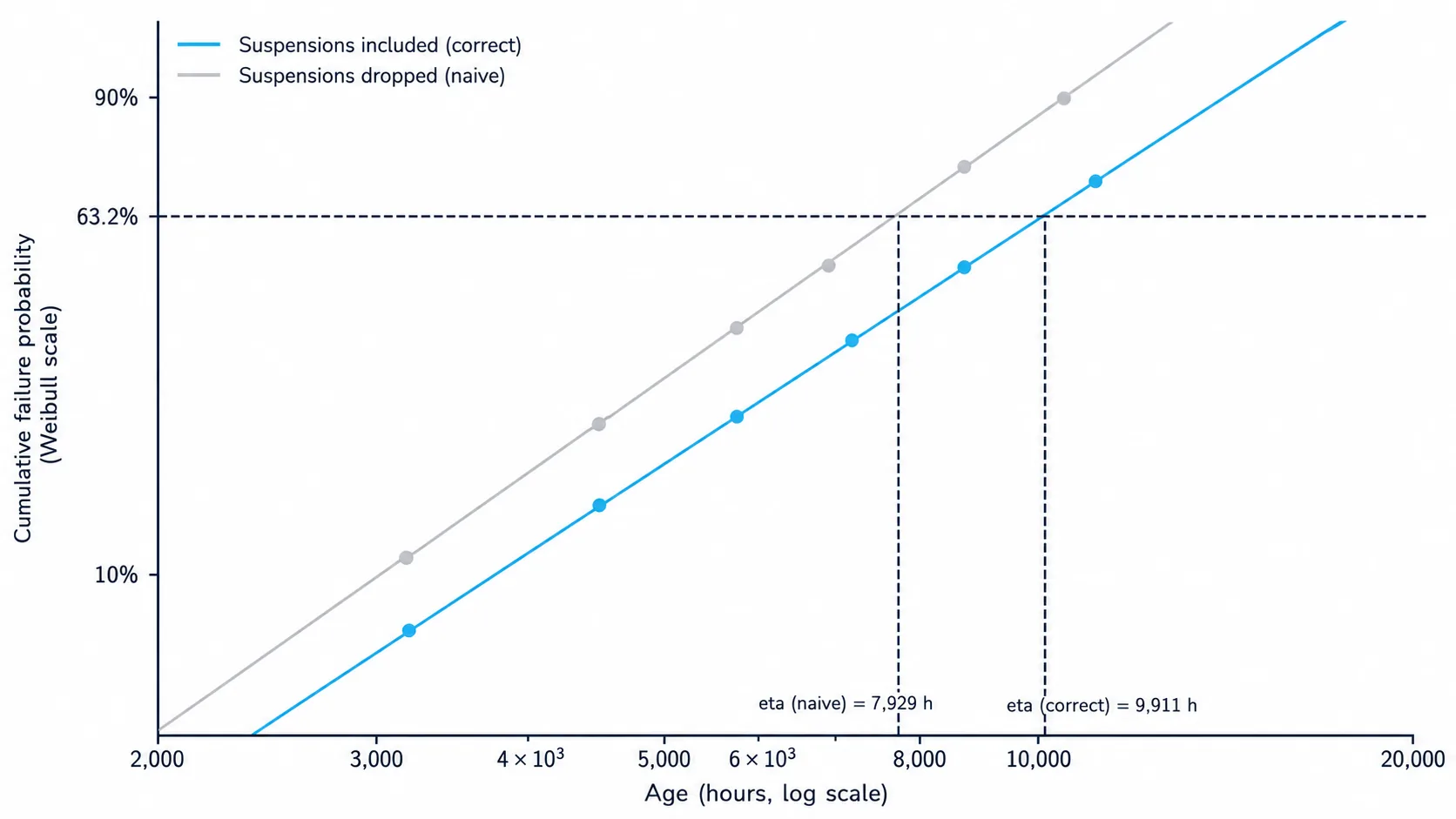
Every naive plotting position sits well above the correct one, because each failure is credited with a larger share of a population artificially shrunk to six. Fitting a Weibull line through each set makes the consequence concrete: the correctly treated data return β = 2.23 and η = 9,911 hours; the naive treatment, same six failure ages, returns β = 2.37 and η = 7,929 hours. Dropping the suspensions understates the characteristic life by around 1,980 hours, close to 20%, exactly the pessimistic direction the mechanism predicts (Abernethy 2006). Both β figures sit in the same qualitative territory, a rising hazard consistent with a wear mechanism, but the naive η would justify a materially earlier, unnecessarily conservative replacement interval, built on six units instead of the nine the data actually contained.
THE GATE: Life Distribution or Repairable-System Event Process?
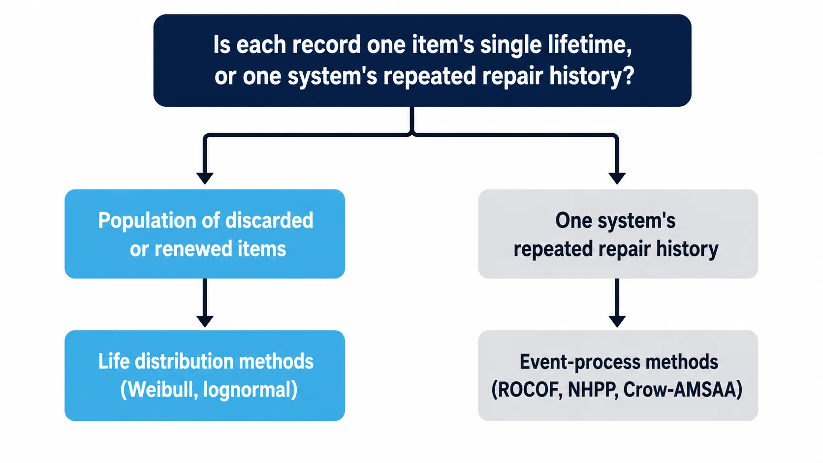
Before any method above is applied, one question decides whether it applies at all: is this data set a sample of lifetimes from a population of comparable items, or a sequence of events on one continuously operating system?
A pump overhauled and returned to service repeatedly over years does not generate a sample of lifetimes; it generates a stream of events on one system. Life distribution methods, the Weibull family among them, need the first kind of data: a population of items, each contributing one lifetime, each discarded or fully renewed at failure. Pool a repairable asset's repair history into that framework anyway, and the method does not fail loudly. It returns a β, an η, a plausible-looking plot, and an answer that describes nothing real, because the object the method assumes was never present in the data.
Telling them apart is a short, practical check:
- Ask what the population actually is. A life-distribution population is a set of distinct items, each contributing exactly one age at failure or suspension. If every row traces back to one physical asset's history, there is no population in the required sense, only one system's timeline.
- Check whether the item is discarded or repaired. A mechanical seal cartridge, replaced whole at failure, is non-repairable in the sense that matters here even if the pump around it is not; the seal never returns to the data set a second time. A gearbox overhauled and returned to identical service is repairable, and its second, third and later failures are not independent draws from a population, they are successive events in one asset's history.
- Route accordingly. A genuine population of discarded or renewed items, one row per item, belongs to life-distribution methods and everything the rest of this series builds on. A repair history on one continuously operating system belongs to event-process methods: rate of occurrence of failures, the non-homogeneous Poisson process, and the Crow-AMSAA power law among them (MIL-HDBK-338B 1998), a distinct, well-established body of technique with its own diagnostic plots and assumptions, genuinely useful and genuinely a different question from the one this series answers.
The same distinction shows up in a metric practitioners already carry: MTBF belongs to a repairable item's event stream, MTTF to a non-repairable item's life distribution. Swapping the two is the same class of error as fitting a Weibull to pooled repairable-system data, worth remembering when a vendor's MTBF claim arrives without a stated basis, since the number is only as meaningful as the population and repair policy behind it.
One Failure Mode, One Data Set
The seal fleet example above tracked one failure mode throughout: seal face wear. Had some of those pumps also suffered O-ring extrusion failures, mixing both modes into one plot would not average cleanly. Each mode has its own hazard mechanism and, in general, its own β and η, and a plot built from mixed modes typically shows as a bend or corner rather than a clean straight line. The fix is to separate the modes and analyse each on its own, a diagnosis this series takes up directly on the next Weibull page.
Extracting Life Data From a CMMS
Almost every life data set in industrial reliability work starts as a set of work orders, not a clean table of ages and statuses, and the extraction step is where most of the discipline above either gets applied or quietly skipped.
A usable extraction needs, at minimum: a stable unit identifier, the age at the event on the declared time base, a status classification, the specific failure mode, and the event from which age is measured, since a component replaced mid-life has an age clock that resets at replacement, not at the parent asset's original commissioning date.
The hardest part in practice is rarely the mathematics. It is identifying which work orders represent a genuine functional failure of the target mode, as distinct from planned maintenance, an unrelated repair, or a description too vague to classify with confidence, and that identification depends entirely on the failure coding structure sitting behind the CMMS. Most systems carry the same coding backbone under a different name: SAP calls it the Catalog Profile, IBM Maximo calls it Problem, Cause, Remedy (PCR). Whatever the label, a usable failure code set covers, as a minimum, the maintainable item, the component or part, the failure mechanism, the failure cause, the effect or symptom, and the corrective or default task.
The ISO 14224 standard publishes a failure mode and mechanism taxonomy at an industry level, and it is a genuinely useful starting reference (ISO 14224:2016). Applied directly and unmodified, though, a generic taxonomy tends to work loosely rather than precisely: categories broad enough to cover every pump in every industry are rarely narrow enough to describe how one specific seal design actually fails, and the same effect ends up coded as a failure mode on one work order and a cause on the next, depending on who filled it in. Codes that drift like this stop discriminating between failure types that behave very differently in practice, which defeats the purpose of coding at all.
The fix is to build the code set bottom-up rather than adopt one top-down: start from a clean, asset-specific equipment hierarchy taken down to the maintainable item and component or part level, then run an asset-class-level FMEA against that hierarchy. Because the FMEA is anchored to the real, inherent failure types of each component or part, the failure mechanisms and causes it identifies are specific enough to code cleanly, and the codes generated from that analysis stay CMMS-ready rather than needing constant reinterpretation on the shop floor. Nexaan APM builds this failure code set automatically from the equipment hierarchy and the asset-class FMEA, CMMS-ready from the first export.
Coded work orders only pay off if the codes are checked and corrected before the work order closes, not after. Get that discipline right and failure and bad-actor analysis stops depending on someone reading every work order individually. The same code, applied consistently, brings different teams to the same reading of the same failure data every time, and extracting a life data set from the CMMS becomes a query rather than a research project, which is exactly what makes everything earlier on this page practical to run in the first place.
Getting This Right Is the Whole Foundation
None of the individual rules here are difficult. Choose the time base the mechanism responds to. Classify every observation correctly, including the ones that never failed. Keep suspensions in the analysis and out of the plot. Check the gate before fitting anything. Every later technique in this series, the fit, the plot, the confidence bound, the replacement interval, inherits whatever was decided here. A defensible analysis is not won at the fitting stage; it is won, or lost, before a single distribution is fitted at all.
Frequently asked questions
What is censored data in reliability analysis?
An observation is censored when the unit is genuinely part of the data set but its failure time is only partly known. There are four recognised kinds. Right censoring, also called a suspension, means the unit has not failed by the target mode at its last observed age. Left censoring means the unit is known to have failed before a certain age but the exact age is unknown. Interval censoring means the failure is known to lie between two inspection points. Truncation is a different problem: the sampling process never lets certain units into the data set at all.
What is the difference between censoring and truncation?
Censoring means a unit is in the data set with incomplete information about its failure time. Truncation means the sampling process never lets certain units into the data set at all. A CMMS that only retains work order history for the last three years will never show a unit that failed and left service before that window began. That unit is not censored, it is truncated out of the sample, and treating a truncated data set as though it were only right-censored understates how much early failure history has actually gone missing.
Why must suspensions be kept in a life data analysis?
A suspension tells you the unit survived to at least its recorded age, and that is real survival information, not an absence of information. Dropping suspensions and analysing only the failures as if they were a complete sample understates the population actually at risk, so every failure looks like it represents more of the fleet than it does, which pushes the fitted distribution toward an earlier apparent failure age. In the worked comparison on this page, the correctly treated nine-unit data set returns a characteristic life of 9,911 hours against 7,929 hours with the suspensions dropped, an understatement of around 1,980 hours.
When should life distribution methods not be used on failure data?
When the data set is a sequence of events on one continuously operating system rather than a sample of lifetimes from a population of comparable items. Life distribution methods need a population of items, each contributing one lifetime, each discarded or fully renewed at failure. A pump overhauled and returned to service repeatedly generates a stream of events on one system instead, and that belongs to event-process methods: rate of occurrence of failures, the non-homogeneous Poisson process and the Crow-AMSAA power law. Pool a repairable asset repair history into a life distribution and the method does not fail loudly, it returns a plausible-looking plot that describes nothing real.