
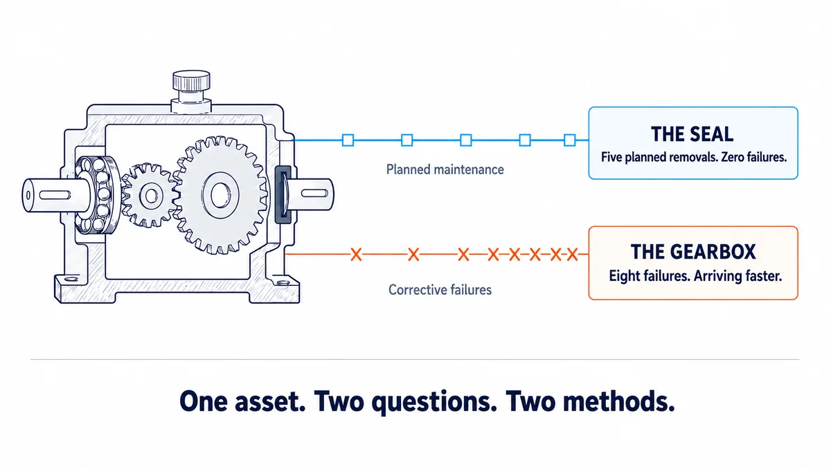
A gearbox seal is replaced every twenty weeks. Nobody on site can say where twenty came from: it predates the current planner, it predates the current maintenance system, and every seal that has come out has come out serviceable. The gearbox itself, meanwhile, keeps coming back, and lately it has been coming back faster.
That is one asset asking two separate questions, and they need two separate methods to answer. Whether the gearbox is demanding corrective attention more often as it ages is a question about a system that gets repaired and put back into service. At what age a bearing reaches a particular failure mode is a question about a population of items, each of which contributes one life. Confuse the two and the arithmetic still runs. It just describes nothing real.
This page works both, end to end, on one hundred weeks of history from a single gearbox: thirteen events, of which only eight are failures. Every intermediate number is shown, so the whole analysis can be reproduced from the tables on this page before anyone has to trust it on their own asset. The data set is illustrative and the cost rates are illustrative, and both are labelled as such where they appear. The methods are not: they are the standard estimators, applied the way a reviewer would expect to see them applied.
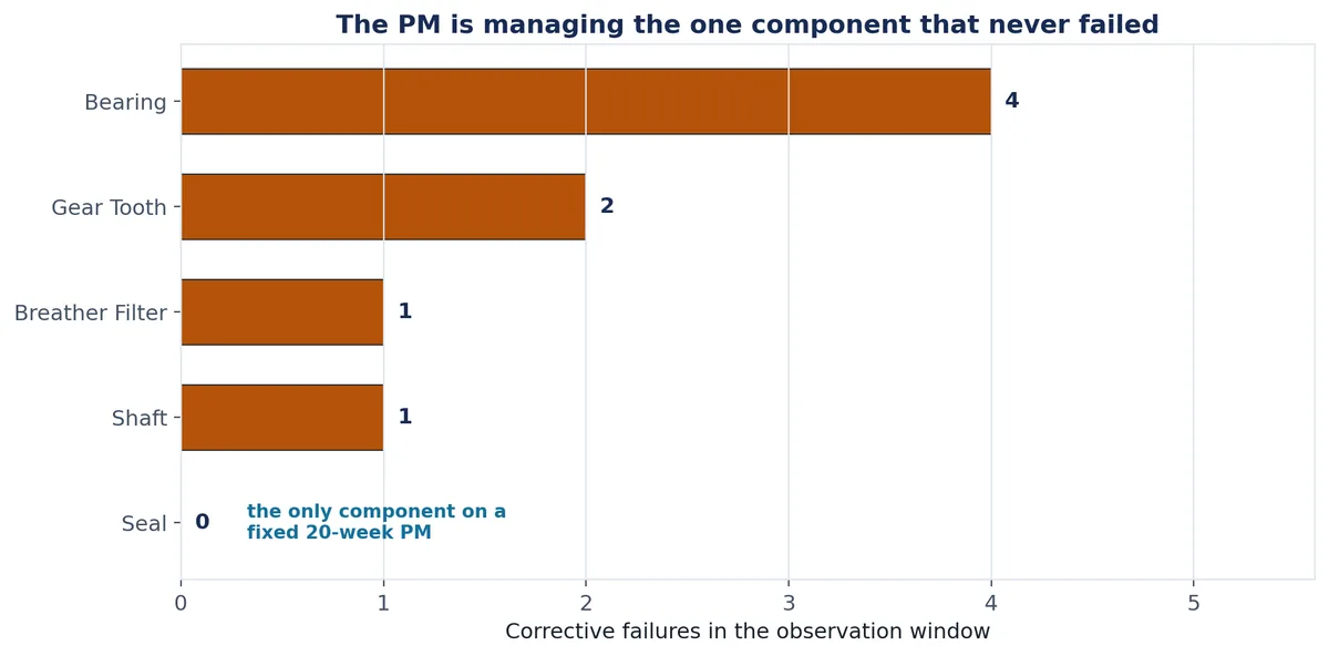
The sentence the analysis ends on is worth stating at the start, because it is what makes the whole exercise worth an afternoon. The only component on this gearbox that is replaced on a fixed interval is the only component that never failed.
The Two Questions One Gearbox Asks
Use Weibull when the item is discarded or renewed at failure, so each unit contributes one lifetime to a population. Use Crow-AMSAA when the same system stays in service after repair and keeps accumulating age, so failures form a sequence of events rather than a sample of lifetimes. The gate is renewal behaviour, not whether the database calls it a component.
That distinction gets lost because the hierarchy label looks like it should settle it, and it does not. A gearbox is a repairable system whether the register calls it equipment, an asset or a maintainable item. A bearing inside it is a non-repairable item, because when it fails it is thrown away and a new one starts at age zero. The same physical machine therefore supports both analyses at once, on different rows of the same history, and running only one of them answers only half the question the site is actually asking. Choosing between life-distribution and event-process methods is worked through in full in Life Data Fundamentals, which sets out the gate, the four kinds of censoring and what each one does to an estimate. The recap here is deliberately short, because the point of this page is what happens after the gate, not the gate itself.
| Weibull | Crow-AMSAA | |
|---|---|---|
| The question it answers | At what age does this item reach this failure mode | Is this system demanding corrective attention more often as it ages |
| What one row of data is | One item, one life, ending in a failure or a suspension | One event on one system, at a cumulative system age |
| What the data must be | Independent, identically distributed lifetimes drawn from one population | An ordered sequence of events on one system that keeps running |
| What happens at failure | The item is discarded or fully renewed, and its clock restarts at zero | The system is repaired and carries on accumulating age |
| What comes out | A life distribution, beta and eta | An event intensity that varies with age, β and λ |
| What beta means | The shape of the hazard rate across one item life | The direction of the trend in event arrivals across the system age |
Both methods produce a parameter called beta, and the two betas do not mean the same thing. A Weibull beta describes the shape of the hazard rate across one item life, so it is a statement about how an individual unit ages. A Crow-AMSAA beta describes the direction of the trend in event arrivals across the system age, so it is a statement about how the whole assembly behaves as a stream of work. Reporting one and calling it the other is a common and expensive slip, and it is worth naming the parameterisation every time a β leaves the analysis.
Thirteen Events, and Only Eight Are Failures
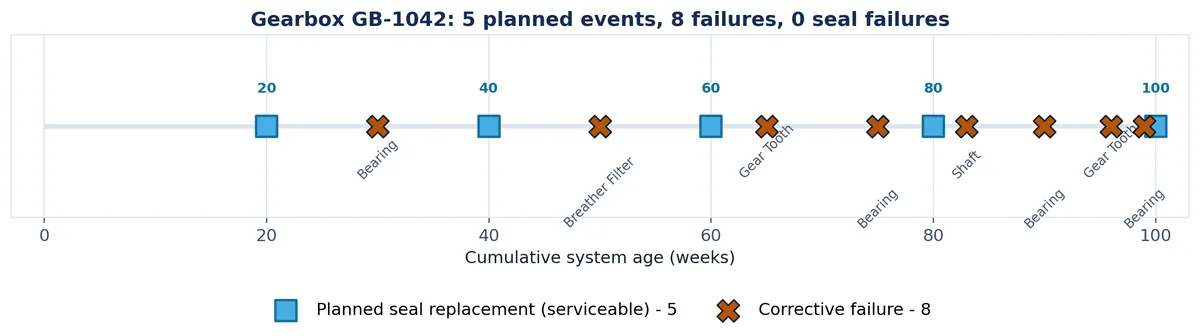
Gearbox GB-1042 was observed from week 0 to week 100. Thirteen events were raised against it in that window: five planned seal replacements at twenty-week intervals, and eight corrective failures. That is the whole history, and the first decision the analysis makes is which of the thirteen belong in the fit.
A planned maintenance work order is not a failure event. Replacing a serviceable gearbox seal every 20 weeks produces five maintenance records over 100 weeks and zero observed seal failures. Including planned removals as failures inflates the event count and corrupts the fitted trend.
The mechanism of the corruption is worth being precise about, because it is not obvious from the output. Adding the five planned removals to the eight failures takes the event count from eight to thirteen and adds events at weeks 20, 40, 60, 80 and 100, which are spread evenly across the window. Evenly spaced events pull a fitted trend toward a constant rate. The analysis would then report a milder trend than the gearbox actually has, on a larger event count that looks like better evidence, and the planned task that caused the distortion would be the thing the report ends up recommending you keep. A work order records work. What it does not record, unless somebody makes it record it, is whether anything had actually failed.
So the inclusion decision is carried as a visible column in the register rather than as a filter applied somewhere upstream, which means the next person to open the file inherits the judgement instead of guessing at it. Getting that column to exist and to be trustworthy across a whole plant is its own body of work, covered in CMMS data quality and failure code integrity.
| System age (wk) | Event type | Component | Failure mode or finding | In the fit |
|---|---|---|---|---|
| 20 | Planned maintenance | Seal | Replaced on plan, found serviceable | No |
| 30 | Corrective failure | Bearing | Bearing Worn due to Inadequate Lubrication | Yes |
| 40 | Planned maintenance | Seal | Replaced on plan, found serviceable | No |
| 50 | Corrective failure | Breather Filter | Breather Filter Blocked due to Dust Ingress | Yes |
| 60 | Planned maintenance | Seal | Replaced on plan, found serviceable | No |
| 65 | Corrective failure | Gear Tooth | Gear Tooth Cracked due to Overload | Yes |
| 75 | Corrective failure | Bearing | Bearing Worn due to Inadequate Lubrication | Yes |
| 80 | Planned maintenance | Seal | Replaced on plan, found serviceable | No |
| 83 | Corrective failure | Shaft | Shaft Worn due to Misalignment | Yes |
| 90 | Corrective failure | Bearing | Bearing Worn due to Inadequate Lubrication | Yes |
| 96 | Corrective failure | Gear Tooth | Gear Tooth Cracked due to Overload | Yes |
| 99 | Corrective failure | Bearing | Bearing Worn due to Inadequate Lubrication | Yes |
| 100 | Planned maintenance | Seal | Replaced on plan, found serviceable | No |
The Terminology the Numbers Depend On
The fourth column of that register is not free text, and the analysis later in this page only exists because it is not. A failure mode is a composite: the component, then the mechanism or state it reached, then the cause that drove it there. Bearing Worn due to Inadequate Lubrication is a failure mode. Worn is a mechanism, and on its own it is not analysable, because four different components can all be worn for four different reasons and a Pareto built on the word returns one meaningless bar.
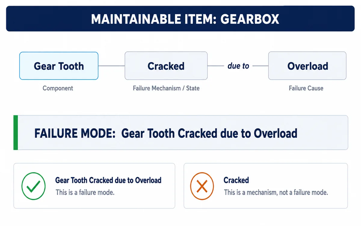
An effect is never a cause, either. The gearbox running hot is what the operator noticed; it is not why the bearing wore. Holding the component, the mechanism and the cause as three separate fields, and assembling the sentence only when it is displayed, is what allows the same history to be counted four different ways later: by component to find where the trend is coming from, by mechanism to find whether one degradation process is running across several components, by cause to find whether one upstream condition is driving all of them, and by full mode to build a strategy. The discipline behind writing modes this way, and turning them into tasks, is the subject of FMECA and RCM as an integrated approach to maintenance strategy.
One more definition has to be nailed down before any of this is fitted, and it is the one most often left implicit. The gearbox is the maintainable item: the level at which work is raised, cost is collected and the event stream is counted. Set that boundary one level too high and the fit pools several machines that do not share a failure process. Set it one level too low and there are not enough events left to fit anything. Where that line sits, and how to make it hold across a site, is the work described in equipment hierarchy development.
The Input People Get Wrong
In a Crow-AMSAA fit, t sub i is the cumulative operating age of the repairable system when the i-th failure occurred, not the interval since the previous failure. Failures at gearbox ages 30, 50 and 65 weeks give t sub 1 equals 30, t sub 2 equals 50 and t sub 3 equals 65.
This is the single most common way the method is fed the wrong quantity, and it is dangerous precisely because both columns are the right length, both are made of plausible numbers, and the estimator returns a β either way. Nothing in the output flags the substitution. The two columns are set side by side in the working table below so the difference is visible: the ages climb from 30 to 99, while the intervals between them fall from 30 weeks to 20, 15, 10, 8, 7, 6 and finally 3.
Those intervals are worth pausing on, because a planner who has lived with this gearbox already knows what they say. Thirty weeks of quiet at the start; three weeks between the last two failures. The eye is not evidence, though, and a run of shortening gaps is exactly the pattern eight random events will sometimes produce by chance. Fitting the trend is what turns the impression into a number. Testing it is what turns the number into an argument, and that comes two sections from now.
Fitting the Power Law
Crow-AMSAA models recurrent failures on a repairable system as a non-homogeneous Poisson process with M of t equals lambda times t to the power beta. β below one means failures are arriving more slowly, β near one means a constant rate, and β above one means the system is deteriorating. It describes the trend, not the cause.
- M of t
- the expected number of events accumulated by system age t
- rho of t
- the instantaneous failure intensity, the rate at which events are arriving at age t
- C of t
- the cumulative intensity, the average rate across the record so far
- lambda
- the scale parameter, which fixes the level of the intensity
- beta
- the shape parameter: below one the system is improving, at one the rate is constant, above one it is deteriorating
The intensity rho of t is an event rate on a system, and it is not the hazard rate of a life distribution even though the two are routinely swapped in conversation. A hazard rate is conditional on one item having survived to an age; an intensity counts events on a system that never resets. The four reliability functions sets out what a hazard rate actually is, which is the fastest way to see why the two are not interchangeable.
One notation warning has to be issued before any β is quoted, because it reverses the meaning of every statement made about the parameter. NIST also writes the power law as M of t equals a times t to the power b, where b plays the role of β here. Some reliability-growth material then defines a growth slope g = 1 − β, and a reader who carries a β from one convention into a sentence written in the other will report improvement where the data shows deterioration. Compare definitions, never symbols, and record the name of the parameterisation alongside the number.
The Estimator, and Every Term in It
For a record with exact event times observed to a fixed end date, the maximum likelihood estimators have a closed form, which is what makes this method workable in a spreadsheet rather than only in software (Abernethy 2006; Crow 1974).
- n
- the number of corrective failures in the window
- T
- the end of the observation window, not the age of the last failure
- t sub i
- cumulative system age at the i-th failure, on one consistent exposure basis
This record is time-terminated: observation ended at T = 100 weeks and the last failure was at week 99, so the window closes on a period of running rather than on an event. The same expression also covers a failure-terminated record, because there the final event sits at T exactly, ln(T / tₙ) is zero, and that term contributes nothing to the denominator. Stating which of the two applies is part of reporting the fit, not a detail: it is what tells a reviewer that the estimator was applied in the form the data called for.
| i | t sub i (system age, wk) | Interval since previous | T over t sub i | the natural log of T over t sub i |
|---|---|---|---|---|
| 1 | 30 | 30 | 3.333333 | 1.203973 |
| 2 | 50 | 20 | 2.000000 | 0.693147 |
| 3 | 65 | 15 | 1.538462 | 0.430783 |
| 4 | 75 | 10 | 1.333333 | 0.287682 |
| 5 | 83 | 8 | 1.204819 | 0.186330 |
| 6 | 90 | 7 | 1.111111 | 0.105361 |
| 7 | 96 | 6 | 1.041667 | 0.040822 |
| 8 | 99 | 3 | 1.010101 | 0.010050 |
| Sum | 2.958147 |
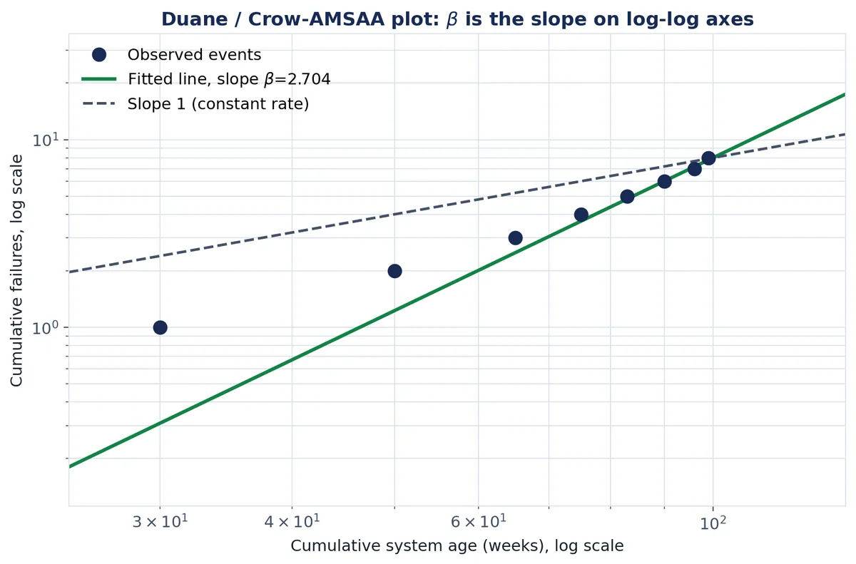
Eight terms sum to 2.9581, which gives a fitted β of 8 divided by 2.9581, or 2.704, and a fitted λ of 8 divided by 100 raised to that power, which is 3.12 × 10⁻⁵. A small-sample correction is available and is dealt with in the next section; the raw estimate is quoted first because it is what the formula returns.
The fit is self-checking, and this is the step most worth building into a template. A correct pair of parameters must reproduce the observed event count exactly, becauseM of T equals lambda times T to the power beta by construction. Here M(100) returns 8.000, against eight observed failures. Any transcription error in the ages, any confusion between the window and the last event, any β carried across from a different asset will break that identity immediately, which is a great deal cheaper than discovering it in a strategy review.
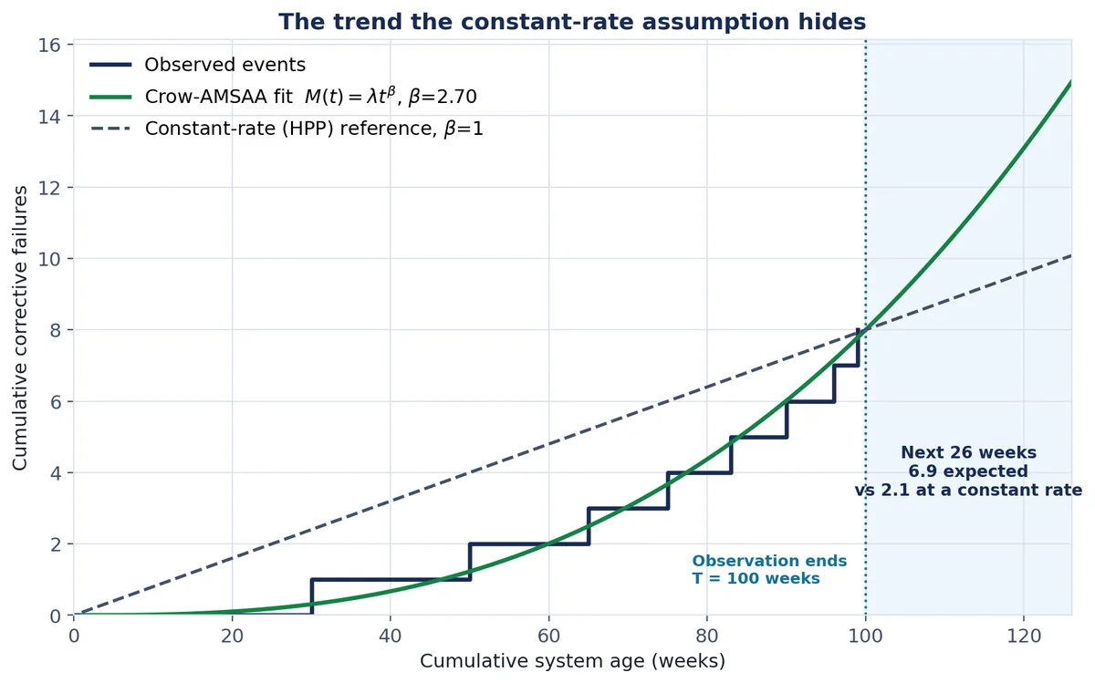
That crossing is the whole argument in one picture. Up to the end of the observation window, a constant-rate assumption and the fitted power law describe the same eight failures, so the two are indistinguishable on the evidence a summary report would show. They separate only in the forecast, which is where every decision actually gets made.
Is the Trend Real, or Is It Eight Points?
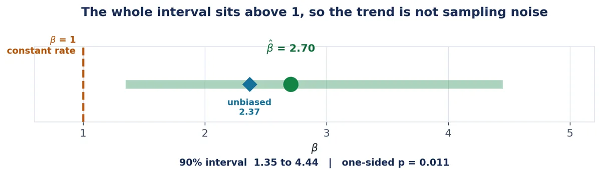
A β of 2.70 is a point estimate from eight events, and on its own it is not evidence of anything. The question a reviewer will ask, and the question that decides whether the finding survives contact with a shutdown-scope argument, is whether a system with a genuinely constant failure rate could have produced this record by chance.
Under the null hypothesis that beta equals one, twice the sum of the natural log of T over t sub ifollows a chi-square distribution with 2n degrees of freedom. For eight failures over 100 weeks the statistic is 5.92 on 16 degrees of freedom, giving a one-sided p-value of 0.011, and a 90 per cent confidence interval on β of 1.35 to 4.44.
- S
- the same denominator sum used by the estimator, 2.9581 for this gearbox
- alpha
- one minus the confidence level, so 0.10 for a 90 per cent interval
Small values of the statistic mean the events are bunching late in the window, which is what deterioration looks like, so the one-sided test in that direction is the one to report. At 0.011 it is comfortably below any conventional threshold, and the 90 per cent interval on β runs from 1.346 to 4.445 without touching one at either end. The 95 per cent interval, 1.168 to 4.876, does not touch one either.
That interval is wide, and honesty requires saying so rather than quoting the point estimate and moving on. β could reasonably be anywhere from about 1.3 to about 4.4, which is the difference between a system deteriorating gently and one deteriorating hard. What the interval does establish, unambiguously, is that all of it sits above one. The direction is settled and the magnitude is not. Eight events are enough to prove that a system is getting worse and not enough to say precisely how fast, and a report that claims more than that from this sample is claiming something the data will not support under questioning.
There is also a small-sample bias to disclose. The maximum likelihood estimate of β runs high on short records, and multiplying by (n − 1)/n gives an unbiased estimate, here 2.366 against 2.704. Both are reported, because the biased estimate is what the formula returns and the corrected one is what a forecast should use. The same asymmetry appears in life-data work, where an overstated shape parameter silently overstates the case for age-based intervention; parameter estimation and confidence bounds works through what small samples do to a fitted β and what a confidence bound is honestly claiming once you have one.
What the Trend Costs
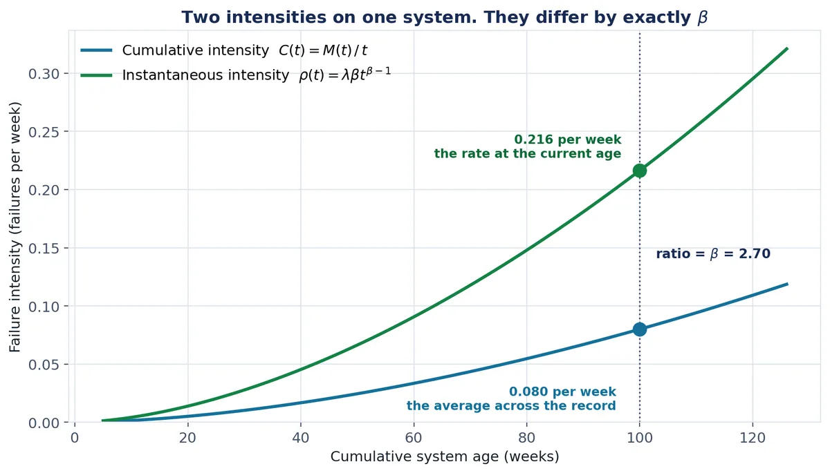
Cumulative intensity is M of t divided by t, the average rate across the whole record. Instantaneous intensity is rho of t equals lambda times beta times t to the power beta minus one, the rate at the current age. They differ by exactly β. A gearbox with a cumulative intensity of 0.080 failures per week and β of 2.70 has an instantaneous intensity of 0.216, nearly three times higher.
That factor is not an approximation and it is not a coincidence. Divide rho of t by C of t and everything cancels except β, at every age, for every fitted power law. It is also the reason the maintenance report and the maintenance planner have been disagreeing about this gearbox for a year, and why both of them are right. The report averages the whole record, so it sees 0.080 failures per week. The planner is living at the right-hand end of it, where the rate is 0.216. Their reciprocals, 12.5 weeks and 4.6 weeks, are the two figures each would recognise as the interval between failures, and the gap between them is β.
Extending the fit past the observation window turns the shape parameter into something a budget conversation can use. Over the next twenty-six weeks the fitted model expects 6.95 further failures. A constant-rate assumption, anchored on the same eight events, expects 2.08. That is an understatement of 3.3 times, on a record both methods agree about up to week 100.
| Crow-AMSAA fit | Constant rate | |
|---|---|---|
| Expected cumulative failures at week 126 | 14.95 | 10.08 |
| Additional failures over the next 26 weeks | 6.95 | 2.08 |
| Age at the ninth failure | 104.5 wk | 112.5 wk |
| Next failure due in | 4.5 wk | 12.5 wk |
| Illustrative exposure over 26 weeks at $18,500 per event | $128,505 | $38,480 |
The probability statement is the one that tends to land in a planning meeting. Substituting into the zero-event expression for the interval from week 100 to week 113 gives 0.044, so there is roughly a four per cent chance of getting through the next quarter without a corrective failure on this gearbox. Over four weeks the odds are much better, at 0.409. Over the full twenty-six weeks they collapse to 0.001.
Priced at an illustrative $18,500 per corrective event, the fitted trend carries $128,505 of exposure over those twenty-six weeks against $38,480 on the constant-rate assumption. Those rates are illustrative and should be replaced with the site's own before the number is quoted anywhere. What does not change with the rate is the ratio, and the ratio is the finding: a constant-rate assumption on this gearbox understates the next two quarters by a factor of three, and the shortfall is invisible in any report that only looks backwards. Which of those events actually matters, and how hard, is a consequence question rather than a rate question, and that is what asset criticality analysis exists to answer.
What Beta Does Not Tell You
A fitted beta above one is a statement about the arrival rate of events on one system. It names no component. It identifies no failure mechanism. It carries no cause, and it prescribes no task. Crow-AMSAA is not root cause analysis and it is not a maintenance strategy method, and treating a β of 2.70 as an instruction to replace or overhaul something is the fastest way to spend money on the wrong component and then conclude that the analysis did not work.
What it does tell you is that this gearbox is worth an hour of somebody's attention, roughly how urgently, and that whatever is driving it has been getting stronger across the window rather than sitting still. That is a genuinely useful thing to know and it is the beginning of the work, not the end of it. The rest of this page is the drilldown the trend demands.
The Drilldown the Trend Demands
Counting the eight failures by mode takes about a minute and changes the whole shape of the conversation.
| Failure mode | Count | Share |
|---|---|---|
| Bearing Worn due to Inadequate Lubrication | 4 | 50.0% |
| Gear Tooth Cracked due to Overload | 2 | 25.0% |
| Breather Filter Blocked due to Dust Ingress | 1 | 12.5% |
| Shaft Worn due to Misalignment | 1 | 12.5% |
| Seal, any mode | 0 | 0.0% |
Half of every corrective failure on this gearbox is one mode: Bearing Worn due to Inadequate Lubrication. The seal, which is the only component carrying a fixed replacement interval, appears nowhere, because it has never failed. Whatever the twenty-week task is achieving, it is not preventing any of the eight events that actually happened.
There is a second pattern in the register that the Pareto alone does not show, because it depends on the order rather than the count. The breather filter blocked at week 50, from dust ingress. Before that event there had been one bearing failure, at week 30. After it there were three, at weeks 75, 90 and 99, with the gaps between them running 45 weeks, then 15, then 9.
A blocked breather lets a gearbox breathe through its seals instead, which draws contamination into the oil, and contaminated oil is a lubrication problem. That sequence is consistent with the record and it is worth an oil sample and a breather inspection this week. It is not a proven root cause, and it should not be written up as one. One event is not a trend, four bearing failures is a small sample, and the same shortening pattern would appear if the duty had changed at around the same time for a reason nobody logged. State it as a hypothesis the evidence supports, name the two checks that would confirm or kill it, and let the oil sample settle it. The credibility of everything else on the page rests on not over-claiming here.
The Seal: Zero Failures Is Not Zero Information
Five components removed serviceable at 20 weeks are five right-censored observations, not five failures. With β assumed at 2 and 90 per cent confidence, Weibayes puts characteristic life at 29.5 weeks or more. The classical zero-failure substitution is a one-sided 63 per cent lower confidence bound, not a point estimate.
With no failures at all, β and η cannot both be recovered from the data, because there is nothing in the record that carries information about the shape. Weibayes resolves that by fixing β from engineering judgement and using the accumulated exposure to put a lower bound on η. The assumption does not go away; it becomes explicit, auditable and arguable, which is the entire value of the method.
- eta lower
- the one-sided lower confidence bound on characteristic life
- beta
- assumed from engineering judgement, never fitted from this data
- C
- the confidence level the bound is stated at
Five seals, each surviving twenty weeks, give a summed exposure of 2,000 when β is assumed to be 2. At 90 per cent confidence the bound comes out at 29.5 weeks, against a replacement interval of 20. The seal is being taken out, on the evidence available, somewhere around two thirds of the way to a conservative lower bound on its characteristic life.
| Assumed β | Confidence | sum of t to the power beta | η is at least (wk) | B10 is at least (wk) |
|---|---|---|---|---|
| 1.0 | 63.2% | 100 | 100.03 | 10.54 |
| 1.0 | 90% | 100 | 43.43 | 4.58 |
| 1.0 | 95% | 100 | 33.38 | 3.52 |
| 2.0 | 63.2% | 2,000 | 44.73 | 14.52 |
| 2.0 | 90% | 2,000 | 29.47 | 9.57 |
| 2.0 | 95% | 2,000 | 25.84 | 8.39 |
| 3.0 | 63.2% | 40,000 | 34.20 | 16.15 |
| 3.0 | 90% | 40,000 | 25.90 | 12.23 |
| 3.0 | 95% | 40,000 | 23.72 | 11.20 |
Publishing the whole table rather than the single headline is deliberate, because the table makes a point the number cannot. At 90 per cent confidence the answer moves from 25.9 weeks to 43.4 weeks purely on which β is assumed, and β here is a judgement about how seals wear, not a measurement. Anyone who disagrees with the assumption can read their own row off the table and see exactly what their disagreement is worth. That is a far stronger position than a single defended number.
One framing point matters more than any of the figures. The familiar zero-failure shortcut, substituting one failure where none occurred, is equivalent to reading the 63.2 per cent row of that table, and it therefore returns a one-sided 63 per cent lower confidence bound rather than an estimate of characteristic life (Abernethy 2006). Reports that call it the characteristic life are wrong, and the error runs in the optimistic direction. Weibayes deserves a page of its own rather than a section, and it will get one; the treatment here goes as far as this gearbox needs and then stops.
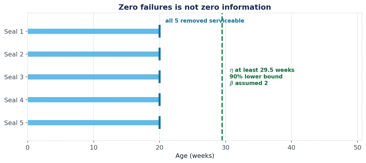
So the original question has an answer. The twenty-week interval is conservative at best, on the only evidence anybody has. Worse, the task is destroying the evidence that would justify it: every seal comes out at exactly twenty weeks, so the data set can never contain a seal life, and the interval can never be tested against anything but a bound derived from an assumption. At an illustrative $1,200 per replacement and 2.6 replacements a year, that is roughly $3,120 a year spent managing a component responsible for none of the eight failures.
What that does not license is stretching the interval to 29.5 weeks, or to any other number. A lower bound on characteristic life is not a replacement interval, and choosing an interval means weighing the cost of the planned task against the cost and consequence of the failure it is meant to prevent. That calculation is a separate piece of work with its own preconditions, and this page deliberately stops before it. The question answered here is whether the task is doing anything, and the answer is that nothing in one hundred weeks of history suggests it is.
The Bearing: The Right Weibull, and the Trap Beside It
The bearing is the component that has actually been failing, four times, and it is a non-repairable item: each failed bearing is replaced with a new one. So it is a legitimate Weibull candidate, and this is where the second method earns its place on the same asset. The only question is which age to fit.
| Event | System age (wk) | Bearing age (wk) |
|---|---|---|
| 1st bearing failure | 30 | 30 |
| 2nd bearing failure | 75 | 45 |
| 3rd bearing failure | 90 | 15 |
| 4th bearing failure | 99 | 9 |
| Bearing still running at week 100 | not counted | 1, suspended |
The left-hand column is the gearbox's age. The right-hand column is the bearing's age, and it is the only one of the two that describes the item being modelled. Each replacement bearing starts at zero, so the bearing fitted in the second row of that table had been in service for 45 weeks, not 75. There is also a fifth observation that the wrong column loses entirely: the bearing installed at week 99 was still running at week 100, which is a one-week suspension and real survival information.
Fitting both, by median rank regression with Johnson adjusted ranks and Benard median ranks, the way Weibull probability plotting sets it out, gives two very different answers from the same four failures.
| Age basis | Sample | β | η (wk) | B10 (wk) | r² |
|---|---|---|---|---|---|
| Bearing age, correct | 4 failures + 1 suspension | 1.376 | 29.09 | 5.67 | 0.9797 |
| System age, wrong | 4 failures | 1.968 | 85.30 | 27.19 | 0.8761 |
Characteristic life is overstated by 2.9 times and B10 by 4.8 times. A spares plan built on the wrong fit would expect ten per cent of bearings to have failed by 27 weeks when the correct figure is under six, which is the difference between holding a spare and not holding one.
The dangerous part is not the size of the error. It is that nothing announces it. An r² of 0.876 on the wrong fit is not obviously bad; it would survive a glance, it would survive most review meetings, and the plotted points sit on a plausible line. Reading a plot as a diagnostic instrument rather than a decoration is a skill in itself, and reading a Weibull plot covers what curvature, corner points and a suspiciously good correlation are actually telling you. What neither r² nor any goodness-of-fit statistic can detect is that the analyst put the wrong quantity into the age column, because the arithmetic is impeccable either way.
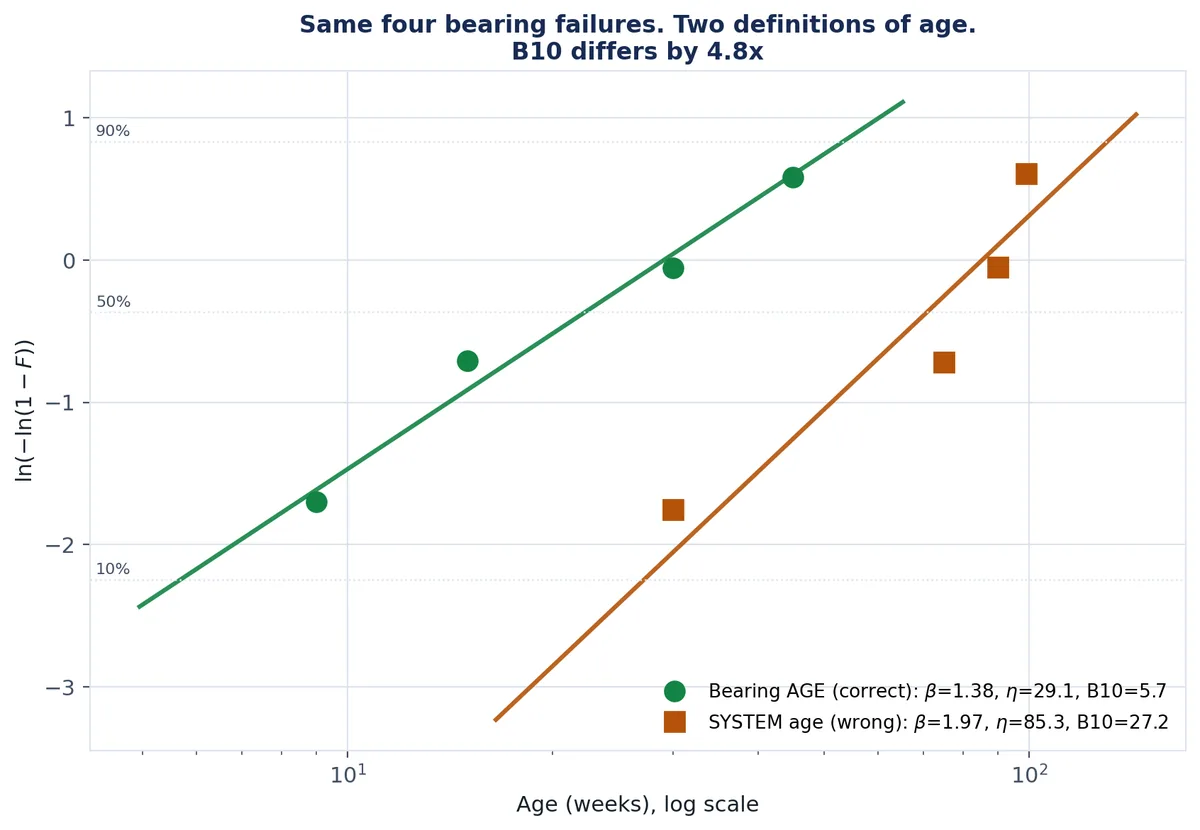
Four failures is a small sample and the fitted β carries real uncertainty, so the durable lesson here is the 2.9 and the 4.8, not the specific parameter values. What β and η physically control, and how much a shape parameter from four points can be leaned on, is worked through in the Weibull distribution explained.
Why the System-Level Fit Had to Come First
There is a deeper problem with the correct bearing fit, and noticing it is what makes the two halves of this page one argument rather than two.
The correct bearing lives, in the order they occurred, are 30, 45, 15 and 9 weeks. They are shortening. A Weibull assumes lifetimes are independent and identically distributed draws from one population, which means it assumes the order of the values carries no information. Here the order carries almost all of it. These bearings are probably not getting worse as components; the environment they run in is degrading, which is consistent with a breather filter blocking at week 50 and letting contamination into the oil.
Averaging those four lives into one distribution destroys the sequence, and the sequence is the only place the deterioration is visible. The Weibull fit returns a β of 1.376, mild wear-out, respectable r², and it is the wrong description of what is happening. The system-level Crow-AMSAA fit sees the deterioration precisely because it never averages anything: it keeps the events in the order they arrived and measures whether they are arriving faster. That is why the system trend is fitted first and the component life second, and it is why a page that only ran the Weibull would have concluded that this gearbox has a slightly worn bearing population and missed the contamination entirely.
What the Analysis Decided
An afternoon of arithmetic on one hundred weeks of history changes what happens next week on this gearbox, and none of the changes are the one the site expected.
The seal task is not the lever. It is aimed at the only component with no failures against it, it costs roughly $3,120 a year on illustrative rates, and it is destroying the evidence that would let anyone test it. It should not simply be extended, either: the first question is whether a fixed-interval replacement is a technically appropriate task for that failure mode at all, which is a task-selection question rather than an interval question. The lubrication and contamination path is the lever, on the strength of four of eight failures sharing one mode and a breather filter blocking halfway through the window. The first two actions are an oil sample and a breather inspection, and they cost almost nothing.
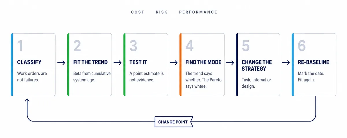
Whatever gets changed, the date it changed has to be recorded, and this is the step most often skipped. A strategy change is a change point in the event process. One power law fitted straight across it averages the deteriorating period and the improved period together and reports something in between, which is a smaller improvement than actually occurred, on data that now describes two different systems. Fit up to the change point, change the strategy, then start a new fit from that date. Otherwise the analysis quietly hides the benefit of the only decision it prompted.
One thing this analysis deliberately did not do is calculate an optimal replacement interval for anything. Establishing that a task is not earning its place is a different question from deciding what the interval should be, the second question needs a cost model and a demonstrated increasing hazard rate on the item itself, and collapsing the two is how a defensible finding turns into an indefensible recommendation.
Run This on One Asset Family
The whole method is eight steps, and on a single asset with a clean event history it is an afternoon's work. Each step below is one action, with the reason it earns its place, because a step followed without its reason is the one that gets dropped first when the analysis is repeated by somebody else.
Classify every event before counting anything, and record the inclusion decision as a visible column rather than a filter someone remembers applying.
A work order records work, not failure, and the difference between the two is the single largest source of corrupted repairable-system analysis; making the decision visible means the next analyst inherits the judgement instead of guessing at it.
Fix the exposure basis and the observation window before fitting, and state whether the record is time-terminated or failure-terminated.
The estimator divides by the observation window, so an ambiguous end date changes every number that follows it, and the termination type is what tells a reviewer which form of the estimator was used.
List the corrective failures at cumulative system age, never as the interval since the previous one.
The estimator takes the ratio of the observation window to each failure age, so feeding it intervals produces a plausible number from the wrong quantity, and nothing in the output signals the substitution.
Fit the power law, then check that the fitted model reproduces the observed event count exactly.
A correct parameter pair must return M(T) equal to n by construction, which makes the fit self-checking and catches a transcription error before it reaches a strategy review.
Test the fitted shape parameter against a constant rate, and report the confidence interval alongside the point estimate.
A point estimate above one is not evidence on its own, and the interval is what separates a trend the data supports from a pattern eight events could produce by chance.
Convert the fitted intensity into expected events over a stated horizon, and attach the consequence those events carry.
A shape parameter does not fund anything; expected events over the next planning window, priced at the site rate, is the form the argument has to take to survive a budget conversation.
Pareto the failure modes to find where the system trend is coming from, and state any causal chain as a hypothesis rather than a conclusion.
The fitted trend says the system is deteriorating but never says which component or why, and over-claiming a root cause on a handful of events costs more credibility than the finding is worth.
Fit component lives on item age rather than system age, and record the date of any strategy change as a change point.
System age silently overstates component life whenever items are replaced during the window, and one power law fitted across a strategy change hides the improvement the change was made to produce.
Everything needed to repeat those eight steps on your own asset is in the analysis pack: the script, the worked data set and a blank event register. The Get the analysis pack button on this page will send it to you. Point it at one asset family and you will know whether the failures are trending and whether the PM task is earning its place.
Where This Gets Hard at Fleet Scale
Doing this on one gearbox is an afternoon. Doing it across a fleet means fixing the failure definition, the exposure basis, the asset boundary and the strategy-change log before any of it can be automated. The method does not change at scale. The governance around it does, and that is where the work actually is.
Staggered installations mean twenty machines all sitting at different system ages, so a pooled fit has to be built from each unit's own age clock rather than from calendar dates. Exposure needs normalising when the units run at different duties, because a week is not a week if one machine runs one shift and another runs three. Major overhauls raise a genuinely hard question about whether the system age resets, is unchanged or lands somewhere in between, and the answer has to be a stated policy rather than a per-analyst decision. Rotable components move between parent assets and take their own age with them, which breaks any assumption that a component's history belongs to the machine it is currently fitted to.
Then there are the two that quietly ruin more fleet analyses than all of the above. Failure definitions drift: what got coded as a failure five years ago is not what gets coded as one now, and a fitted trend across that boundary is measuring a coding change. And strategy changes go unlogged, so change points that should have split the record are invisible and the fit averages across them. Neither is a modelling problem. Both are data governance problems, and both have to be settled before a fleet-wide number means anything.
The Minimum Data Structure
Everything on this page came out of one event register, and the register does not need to be elaborate. What it needs is for a small number of things to be separable, because each separation is what makes one of the analyses possible.
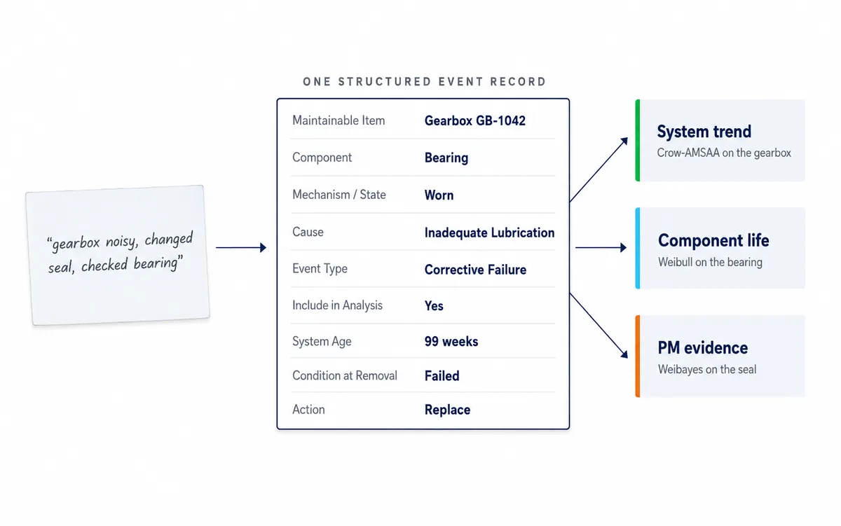
Planned work has to be separable from corrective work, or the Crow-AMSAA fit is counting maintenance instead of failures. The component has to be separable from the mechanism and from the cause, or the Pareto returns nothing usable. Cumulative system age has to be recorded on one consistent exposure basis, or the estimator is fed intervals dressed as ages. The condition found at removal has to be recorded, because serviceable and failed are the difference between a suspension and a failure and nothing else in the record distinguishes them. And the inclusion decision itself has to be a column, so that a fit can be reproduced by somebody who was not in the room when it was made.
Nine fields carried all three analyses on this page. A free-text note reading gearbox noisy, changed seal, checked bearing carries none of them, and no amount of downstream cleverness recovers what was never written down. Building the coding structure that makes those fields reliable across a site is the subject of CMMS data quality and failure code integrity, and the boundary question of what counts as one maintainable item belongs to equipment hierarchy development.
One standing caveat applies to everything above, and it is stated once here rather than repeated in every section. The worked example on this page is an illustrative teaching template, not production calculation software. The data set is illustrative, the cost rates are illustrative, and any real-asset cost, risk, safety, warranty or capital decision taken on the back of these methods needs qualified engineering review.
Frequently asked questions
When do you use Weibull and when do you use Crow-AMSAA?
Use Weibull when the item is discarded or renewed at failure, so each unit contributes one lifetime to a population. Use Crow-AMSAA when the same system stays in service after repair and keeps accumulating age, so failures form a sequence of events rather than a sample of lifetimes. The gate is renewal behaviour, not whether the database calls it a component.
What is t sub i in a Crow-AMSAA fit?
In a Crow-AMSAA fit, t sub i is the cumulative operating age of the repairable system when the i-th failure occurred, not the interval since the previous failure. Failures at gearbox ages 30, 50 and 65 weeks give t sub 1 equals 30, t sub 2 equals 50 and t sub 3 equals 65.
Does a planned maintenance replacement count as a failure?
A planned maintenance work order is not a failure event. Replacing a serviceable gearbox seal every 20 weeks produces five maintenance records over 100 weeks and zero observed seal failures. Including planned removals as failures inflates the event count and corrupts the fitted trend.
What does beta mean in Crow-AMSAA?
Crow-AMSAA models recurrent failures on a repairable system as a non-homogeneous Poisson process with M of t equals lambda times t to the power beta. β below one means failures are arriving more slowly, β near one means a constant rate, and β above one means the system is deteriorating. It describes the trend, not the cause.
How do you test whether a Crow-AMSAA trend is real?
Under the null hypothesis that beta equals one, twice the sum of the natural log of T over t sub i follows a chi-square distribution with 2n degrees of freedom. For eight failures over 100 weeks the statistic is 5.92 on 16 degrees of freedom, giving a one-sided p-value of 0.011, and a 90 per cent confidence interval on β of 1.35 to 4.44.
What is the difference between cumulative and instantaneous failure intensity?
Cumulative intensity is M of t divided by t, the average rate across the whole record. Instantaneous intensity is rho of t equals lambda times beta times t to the power beta minus one, the rate at the current age. They differ by exactly β. A gearbox with a cumulative intensity of 0.080 failures per week and β of 2.70 has an instantaneous intensity of 0.216, nearly three times higher.
What can zero failures prove about a component?
Five components removed serviceable at 20 weeks are five right-censored observations, not five failures. With β assumed at 2 and 90 per cent confidence, Weibayes puts characteristic life at 29.5 weeks or more. The classical zero-failure substitution is a one-sided 63 per cent lower confidence bound, not a point estimate.
Can Crow-AMSAA tell you which component to fix?
No. A fitted beta above one is a statement about the arrival rate of events on one system. It names no component, identifies no failure mechanism, carries no cause and prescribes no task. It tells you the system is worth investigating and roughly how urgently. What to do about it comes from the failure-mode drilldown that follows, and from a maintenance strategy method built for task selection.
If a preventive maintenance interval on your plant has no written basis, or a fitted trend has to survive a shutdown-scope argument, we would be glad to work through one asset family with you.
Start the conversation