
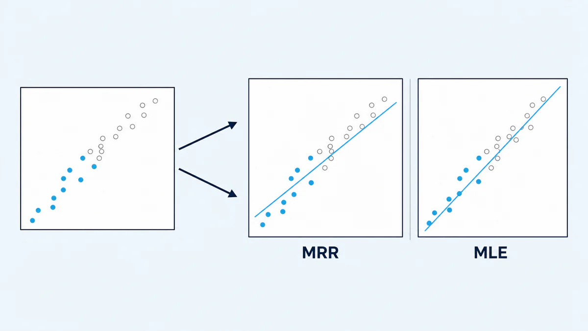
Hand the same life data to two competent reliability engineers and ask each for beta and eta, and you can get back two different answers. Neither has made a mistake. The difference is method, and method is a choice with rules behind it, not a coin toss.
This page sets median rank regression directly against maximum likelihood estimation: how each one actually works, where each is the stronger choice, what a small sample does to a fitted beta, and what a confidence bound is honestly claiming once you have one. Reading a Weibull plot, covered in the previous page in this series, tells you whether a fit is trustworthy. This page tells you how that fit was built in the first place, and how to defend the number that came out of it.
The short version: there is no single correct estimator, only a correct disclosure. State the method, the sample size and the censoring pattern, and the result becomes reproducible by anyone who checks your work.
How Median Rank Regression Works
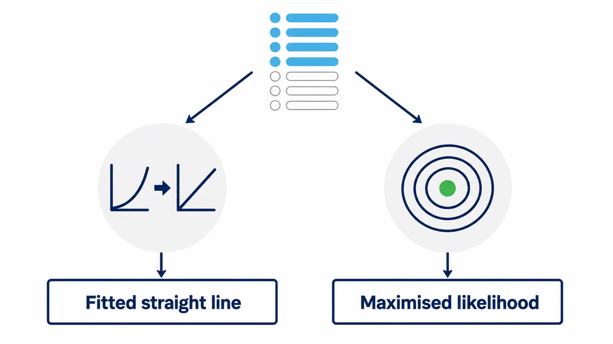
Median rank regression, MRR, is the method behind the step-by-step plotting procedure built earlier in this series and the plot-reading skill built directly after it. It treats the plot itself as the model: transform the data, fit a straight line, and read beta and eta off the line's slope and crossing point. Every worked fit shown so far in this series, including the fleet with the hidden second failure mode two pages back, was produced this way.
- F of t
- the cumulative fraction failed by age t, estimated at each failure by its median rank
- beta
- the shape parameter, read as the slope of the fitted line
- eta
- the characteristic life, read at the point the fitted line crosses 63.2%
- t
- age at each failure, on the declared time base
The transform turns the Weibull's curved cumulative distribution into a straight line on the right axes (Abernethy 2006), and least squares finds the line that sits closest to the transformed points. Two things follow directly from that construction. First, the regression direction is a declared convention, not an arbitrary detail: fitting life on probability and fitting probability on life are both legitimate least-squares problems, and they return slightly different answers on the same data, which is why the direction has to be stated every time. Second, and this is MRR's real advantage, the plot is the deliverable as much as the parameters are. A dogleg, a corner point or a batch signature shows up visually before it shows up as a poor fit statistic, which is why MRR remains the right first move on almost any new data set even when the final reported estimate comes from elsewhere.
How Maximum Likelihood Works
Maximum likelihood estimation, MLE, asks a different question. Instead of fitting a line to transformed points, it asks which beta and eta make the data actually observed the most probable outcome, given the model.
- log-likelihood of beta and eta
- the log-likelihood, the quantity MLE maximises over β and η
- D
- the set of exact failures, each contributing its probability density f(tᵢ)
- C
- the set of suspended (right-censored) units, each contributing only its survival probability S(tⱼ)
- beta and eta
- the shape and scale parameters, the two unknowns being solved for
Every exact failure contributes what it actually tells you, its density at the observed age. Every suspension contributes what it actually tells you and nothing more, the fact that the unit survived to that age, without pretending it will fail at some assumed future point (Abernethy 2006). That is the structural reason MLE handles heavy censoring more gracefully than a plot ever can: a suspension contributes directly to the likelihood through its survival term, while a failure contributes its density, rather than the suspension being excluded from the fitted points and only indirectly adjusting the ranks around it. For a fixed beta, eta has a closed form; beta itself has none and is found by a numerical search on the score equation, which is why MLE needs a solver where MRR only needs a ruler. That search is well behaved for the ordinary case of exact failures plus right suspensions and converges quickly, though a data set with only one failure and several suspensions can leave the solver searching a very flat surface, a case this series returns to directly on the next page.
Choosing Between Them
Neither method is the default, and treating one as the house style regardless of the data is itself a source of avoidable disagreement. The choice depends on what the sample looks like, how it was censored and what the resulting number is actually going to be used for.
| Situation | Favours | Why |
|---|---|---|
| Small sample, and the plot itself is part of the deliverable | MRR | The visual diagnostic value is highest exactly when you have the fewest points to work with, and MRR gives you that plot for free |
| Larger sample, heavy or awkward censoring | MLE | The likelihood treats every suspension on equal footing with every failure, so heavy censoring degrades an MLE fit far more gracefully than it degrades a set of plotting positions |
| The estimate feeds a further calculation | MLE | A replacement-interval or confidence-bound calculation downstream is better served starting from the estimator built for statistical inference, not the one built for visual diagnosis |
| Diagnosing mixed modes, corner points or batch effects | MRR | This is a plot-shape problem, and only a plot answers it |
Abernethy's own guidance is to run both wherever the decision matters, treat agreement as reassurance and treat disagreement as information about the sample, not as a sign that one method has failed (Abernethy 2006). That guidance is the correct answer to the two-analysts problem this page opened with: agreement is not required for either result to be defensible, and a method stated alongside the number is what makes the result reproducible.
Record the sample size, the number of exact failures, the number of suspensions and how those suspensions arose, before choosing an estimator.
The choice in the table above depends entirely on these facts, and a method chosen before the data is characterised is a guess dressed up as a decision.
Fit MRR, MLE or both, using the guidance above to decide which is the primary reported result.
Running both where the decision matters turns disagreement into information about the sample instead of a hidden discrepancy.
If MLE was used on fewer than about twenty failures, flag that the reported beta is susceptible to upward bias on average and note the small-sample limitation explicitly.
An unflagged, overstated beta silently overstates the case for age-based intervention downstream.
State the estimator, the sample size and the censoring pattern alongside every reported beta, eta or B-life.
This is the disclosure that lets another engineer reproduce the result, and it is what actually resolves the two-analysts problem, not agreement between methods.
What Small Samples Do to Beta
MLE has one well-documented weakness that matters more than any of the guidance above: on a small sample, MLE beta is biased high, and the direction of that bias is not neutral.
An overstated beta overstates the case for an increasing hazard rate, which overstates the case for scheduled, age-based replacement. A fleet that genuinely carries a mild wear-out signature can present, on a handful of early failures, as a much sharper wear-out mechanism than the physics actually supports, and every downstream decision inherits that overstatement.
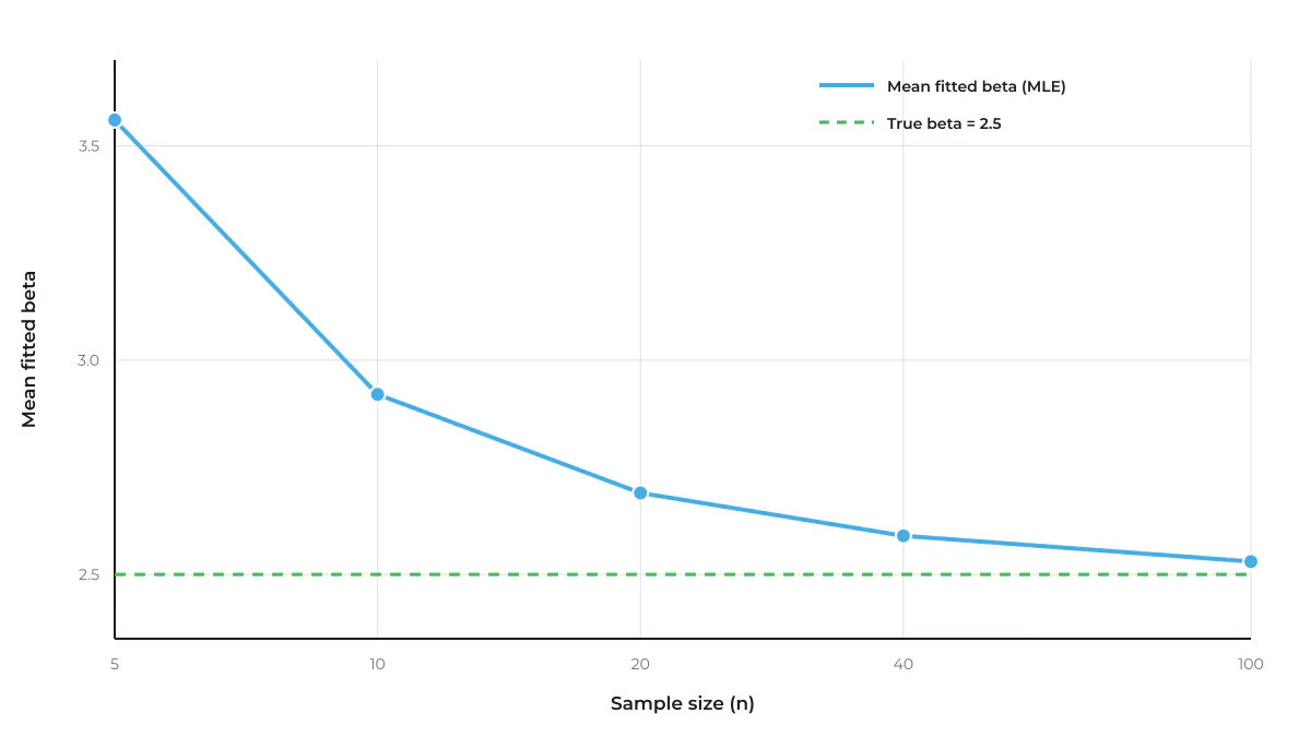
The supplied illustrative simulation shows the size and shape of the effect directly. It draws repeated samples from a known Weibull population (β = 2.5) at several sample sizes and fits each by MLE:
| Sample size | Mean fitted beta | Bias against true beta |
|---|---|---|
| 5 | 3.56 | +42.6% |
| 10 | 2.92 | +16.7% |
| 20 | 2.69 | +7.7% |
| 40 | 2.59 | +3.6% |
| 100 | 2.53 | +1.4% |
The bias is severe at n = 5, still meaningful at n = 20, and effectively gone by n = 100 (Abernethy 2006 reports the same qualitative pattern from an independent historical comparison). The practical rule that follows: treat an MLE beta from fewer than about twenty failures as susceptible to upward bias on average, not as an individual upper bound on the true shape. Report that limitation and weight a replacement-interval decision accordingly rather than taking the point value at face value. A cost-optimised replacement interval, covered later in this series, is only defensible when the hazard rate genuinely increases with age, and an inflated beta from a thin sample can make that precondition look satisfied when a larger sample would not have supported it.
B10, B50 and Why Tail Estimates Are More Sensitive
Beta and eta are rarely the number a business decision actually needs. A B-life, the age by which a stated percentage of the population has failed, is.
- B sub p
- the age by which fraction p of the population has failed
- p
- the stated fraction, expressed as a decimal (p = 0.10 gives B10, p = 0.50 gives B50)
- eta and beta
- the fitted scale and shape parameters
B50 is the median life, useful for describing the fleet in general terms. B10, the age by which 10% have failed, is the figure practitioners reach for most often in spares planning and warranty argument, because it describes early attrition rather than the typical unit, and it is usually the number a procurement or warranty conversation is actually built around (Abernethy 2006). Getting B10 wrong by even a few percent has a real cost on both sides: it understates spares demand and warranty exposure if the true B10 is lower than reported, and it ties up capital in premature stock if the true B10 is higher.
A confidence bound on any of these has to name its target before it names its width. A bound on beta is a statement about the fixed, unknown shape parameter; a bound on a B-life is a statement about a fixed, unknown age; and neither is the same claim as a prediction interval for what a single future unit will do. Two families of method build these bounds: a Fisher-information or delta-method approach, which uses the curvature of the likelihood around its maximum to approximate a variance, and a likelihood-ratio approach, which finds the range of parameter values whose likelihood stays acceptably close to the maximum. Both require declaring the confidence level, the sidedness (a one-sided lower bound is not one end of a two-sided interval) and the method, because none of those three has a silent default.
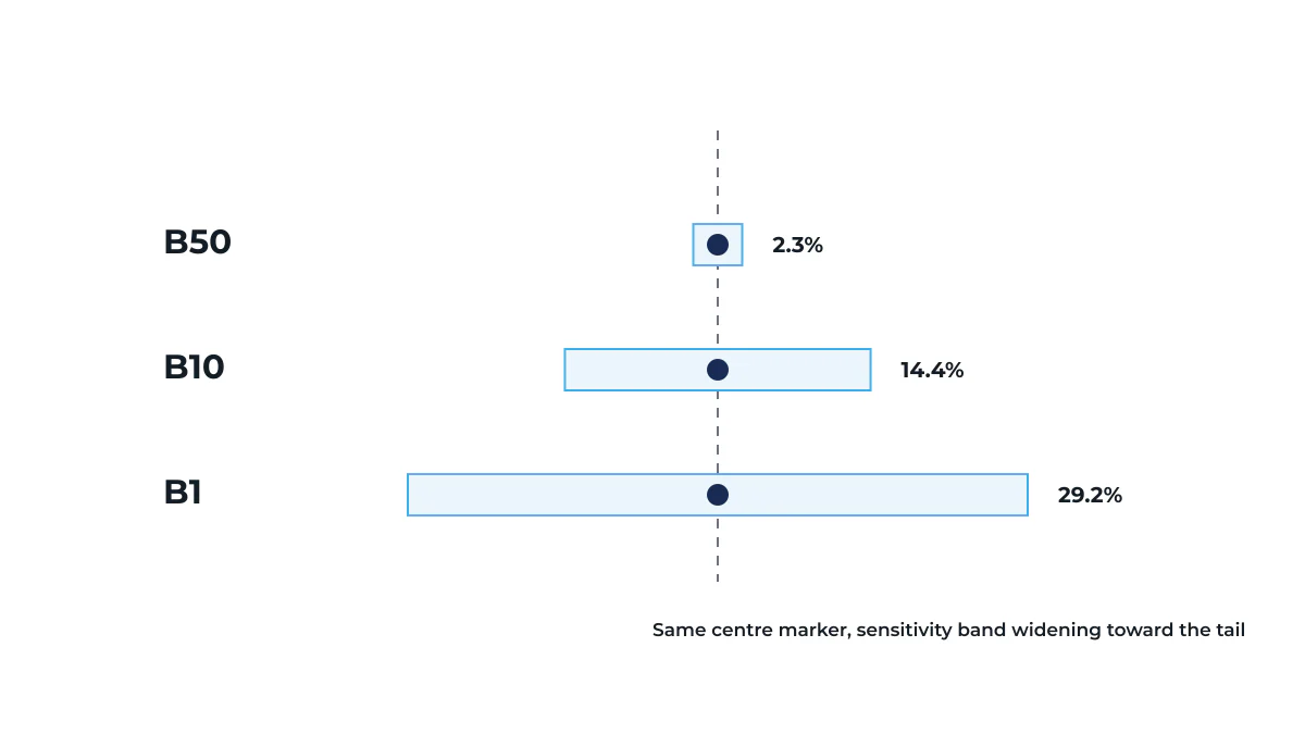
Tail percentiles are also more sensitive to changes in the fitted shape. The following calculation holds eta fixed at 16,075.39 hours and changes beta by ±10% for three B-life targets. It is a beta-only sensitivity check, not a statistical confidence interval: it has no confidence level and does not include uncertainty in eta or beta–eta covariance.
| Target | Point estimate | Range from β ±10% | Range width |
|---|---|---|---|
| B50 | 14,308 h | 14,124 – 14,461 h | 2.3% of the point estimate |
| B10 | 7,864 h | 7,263 – 8,392 h | 14.4% of the point estimate |
| B1 | 3,727 h | 3,169 – 4,257 h | 29.2% of the point estimate |
The same relative change in beta produces a sensitivity range more than twelve times wider, as a share of the point estimate, at B1 than at B50. A tight-looking sensitivity range at the median says nothing about the width of a formal confidence interval at the percentile you are actually trying to defend.
The Same Fleet, Two Methods
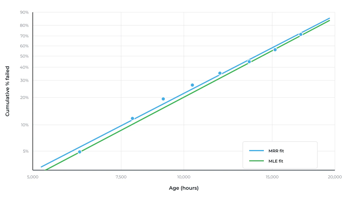
A 14-unit fleet of haul truck final drive planetary bearings puts every point above on one data set: eight failures at 6,200, 7,900, 9,100, 10,400, 11,800, 13,500, 15,200 and 17,100 hours, and six units still in service at 8,500, 11,000, 12,800, 14,600, 16,500 and 18,900 hours.
Fitted by median rank regression using life-on-probability inverse regression—regressing log life on transformed plotting probability and then inverting the slope—with adjusted ranks and Benard's approximation carried across from earlier in this series: β = 3.081, η = 15,690 h, r = 0.9957. Fitted by maximum likelihood on the same fourteen units: β = 3.147, η = 16,075 h.
| Result | MRR | MLE | Difference |
|---|---|---|---|
| Beta | 3.081 | 3.147 | 2.2% |
| Eta | 15,690 h | 16,075 h | 2.5% |
| B10 | 7,558 h | 7,864 h | 4.1% |
| B50 | 13,930 h | 14,308 h | 2.7% |
Neither number is wrong. MRR weights every plotted point equally in the transformed coordinate space; MLE weights each observation, failure or suspension, by its actual contribution to the likelihood, which is a different and equally legitimate way of using the same fourteen bearings. The 4.1% gap on B10, the figure most likely to drive a spares or warranty decision, is exactly the kind of difference that turns into an argument if the method used to produce each number was never stated. State it, and the argument does not start. With eight failures against six suspensions, this fleet sits in the size range where either method is defensible, which is itself the point: the honest answer to "which one is right" is that both are, and the report earns its credibility from naming the method and the sample it rests on, not from picking the number that happens to look cleaner.
What Actually Settles the Disagreement
Two analysts on the same data set are allowed to report different beta values. What they are not allowed to do is report one without saying which method produced it, how many units the estimate rests on, and how those units were censored. That disclosure, not agreement between methods, is what makes a Weibull result something another engineer can check and trust.
The next page in this series turns to the opposite data problem: fleets with only one failure, or none at all, and how Weibayes turns thin data into a defensible lower bound rather than a guess.
If your fleet's fitted beta depends on which method produced it, or a B10 needs to hold up under a spares or warranty argument, we would be glad to work through the analysis with you.
Start the conversation