
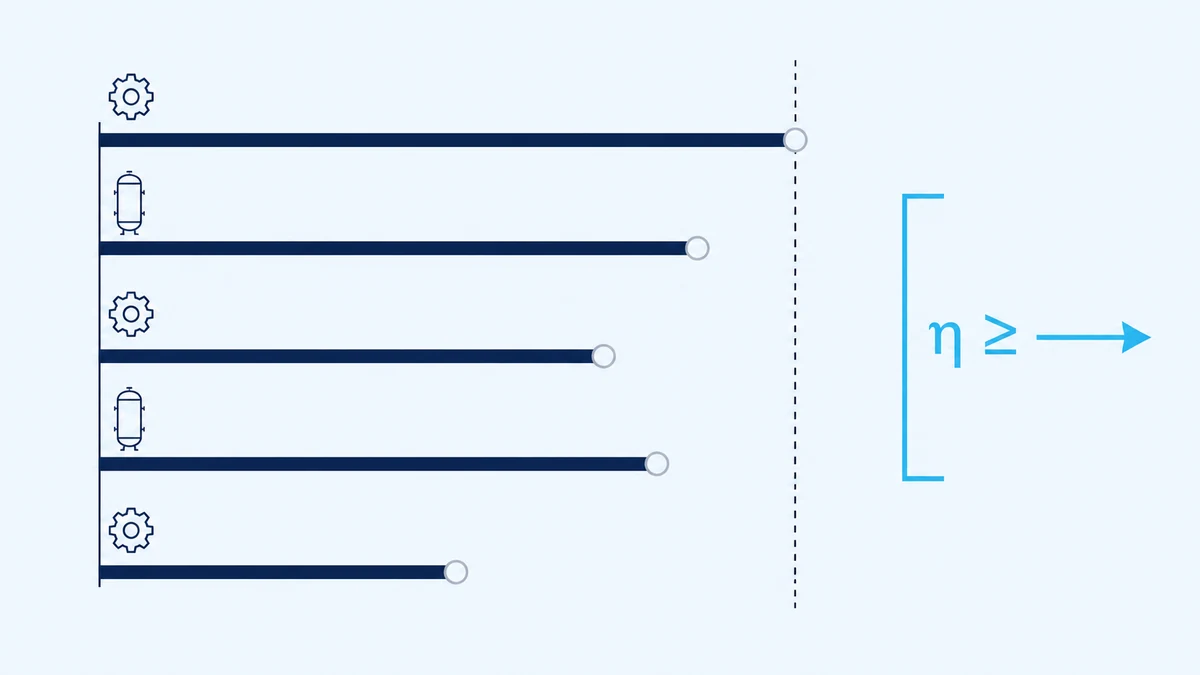
A critical gearbox has run for four years without a single failure. Your manager wants a number before the next shutdown: how much longer can we trust this before it becomes a risk? Every fitting method built earlier in this series needs failures to work, and you have none. That is not a gap in your data. It is the exact situation this page exists to solve.
This happens on every site, on some of the equipment that matters most. A component that almost never fails gives you almost nothing to plot, and the assets with the cleanest run history are usually the ones a shutdown planner or a purchasing manager most wants a defensible number on. Weibayes is the method that turns a clean run history into that number, honestly, without pretending you have more evidence than you do.
Here is what follows. First, why the ordinary fitting methods from earlier in this series produce nothing at zero or one failure. Second, what Weibayes trades to get an answer anyway, and where that trade is legitimate. Third, the method itself, worked step by step on one real fleet. Fourth, what the resulting number actually tells you on site, and what it does not. Fifth, how to size a test on purpose, before an asset is even installed, to prove a target rather than wait for field data to accumulate.
Why Zero Failures Breaks Ordinary Weibull Fitting
Picture trying to draw a trend line through data points. One point does not tell you a slope. Zero points do not tell you anything at all. Weibull fitting has exactly the same problem.
Median rank regression, from earlier in this series, needs failure points to plot a line through. Maximum likelihood needs enough failures to locate a clear best answer among all the possibilities. Take the failures away and both approaches run out of ground to stand on. With zero failures, the calculation that would normally search for the best-fitting characteristic life, eta, keeps improving without limit: a longer assumed life always explains a longer run of survivors slightly better, so the search never settles anywhere and returns no answer at all (Abernethy 2006). With exactly one failure, the search does complete, but it is like fitting that trend line through one data point: many different slopes pass through it almost equally well, so the shape parameter, beta, the number that says whether risk climbs steeply or gently with age, comes out barely more informed than a guess.
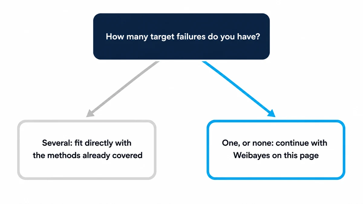
This is not a flaw in the maths. It is the maths correctly reporting that a handful of clean running hours cannot, by itself, answer a two-part question (how steeply does risk climb, and over what timescale). Something has to be supplied from outside the data. Weibayes is the disciplined way to supply it.
What Weibayes Trades for a Usable Answer
Weibayes makes one trade: it takes beta, the shape of how risk climbs with age, as an assumption from outside this data set, and in exchange it can still answer the scale question, how many hours, with real numbers.
That trade is only worth making if the assumed beta is defensible, because every number that follows depends on it. Three sources are legitimate. The physics of the failure mechanism can fix beta directly: a bearing wearing out under rolling-contact fatigue, a tube creeping under sustained heat and stress, or a component corroding under a known chemical attack each has a broadly predictable pattern of risk rising with age, independent of which specific unit you are looking at. A prior Weibull fit on the same failure mechanism in a genuinely comparable population is the most common source in practice: same mechanism, same environment, same duty, only the running hours have changed. Documented industry data for that mechanism, from a source that states its own population and method, is the third (Abernethy 2006).
What is not legitimate is choosing beta because it makes a target look achieved. A steeper assumed beta and a gentler one, applied to the same running hours, can produce noticeably different answers, and a beta chosen after seeing which one clears the bar is not an assumption any more. It is the answer, worked backwards. Weibayes also carries the same rule as every other method in this series: keep failure mechanisms separate. Mixing a bearing's wear-out pattern with a seal's random failures under one assumed beta produces a number with no real mechanism behind it (ISO 14224:2016).
The Method, Step by Step, on a Real Fleet
Here is the fleet this page uses throughout. A refinery has just retubed a crude-unit fired heater, replacing the original alloy with a more heat-resistant one, in three stages as the shutdown schedule allowed: 20 tubes have now run 26,000 hours, 16 have run 23,500 hours, and 12 have run 19,000 hours. None have failed by creep rupture, the slow stretching and eventual splitting that heat and stress cause in a tube wall over years of service. The next major shutdown is 40,000 hours away, and the reliability engineer has been asked one question: are these tubes going to make it?
Creep rupture is well understood on this site from the original alloy's long service history, and the new alloy is expected to resist the same mechanism for longer without changing its basic shape, so a beta of 3.5 is a defensible starting assumption. That single number is what lets the calculation proceed at all.
When You Have At Least One Target Failure
- eta hat
- the estimate of the characteristic life, the age by which 63.2% of the population would be expected to have failed by this mechanism
- t sub i
- the age of every unit at last observation, whether it failed or is still running, all on one consistent time base
- beta
- the assumed shape parameter, supplied from outside this data set
- r
- the number of observed target failures
This is the same estimator this series built for maximum likelihood, with one difference: there, the search found the beta that best explained the data; here, beta is fixed first and only eta is solved for (Abernethy 2006). Every unit's age is raised to the power beta and summed, whether that unit has failed or is still running. A tube still in service at 26,000 hours has accumulated real exposure to the failure mechanism, and it contributes to that sum exactly as a failed unit's age would, because both are answering the same question: how much time-at-risk has this population actually built up.
When You Have None At All
Set r to zero in that formula and it has no answer, which is the correct reflection of the earlier finding: an ordinary estimate genuinely does not exist with zero failures. The usable result instead is a lower bound, a number you can state with a chosen level of confidence rather than a single best guess.
- eta sub L
- the lower bound on the characteristic life, stated at a chosen confidence, not an estimate of it
- alpha
- one minus the confidence level being claimed (alpha of 0.10 states the bound at 90% confidence)
- t sub i and beta
- as above, with every unit here a running survivor, since none have failed
The term −ln α does the same job r did in the first formula: a smaller α, meaning a higher stated confidence, makes −ln α larger, which divides the exposure down further and produces a smaller, more conservative bound (Abernethy 2006). Demanding more confidence always costs some bound. There is no way around that trade, only a choice of how much of it you want.
Confirm and write down where the assumed beta actually comes from: mechanism physics, a prior fit on the same mechanism in a comparable population, or documented industry data for that mechanism.
Every number that follows is conditional on this one choice. A bound built on an undocumented or convenient beta is not defensible, even when the arithmetic behind it is correct.
Raise every unit’s running hours to the assumed beta and add them together, including units that are still running.
A survivor has not stopped contributing information just because it has not failed. Two tubes still running at 20,000 hours each contribute 20,000 raised to the beta, not zero, to that total.
Choose and state a specific confidence level, then apply the lower-bound formula rather than defaulting silently to a bare, unstated convention.
Zero failures is not a separate, special case bolted onto the method. It is the same formula at the one value of r where an ordinary estimate is mathematically impossible, and a bound is the only honest output.
Report the result as exactly what it is: a lower bound at a named confidence, built on a named assumed beta, never as an unconditional finding about the asset’s life.
A reader who sees the number without that qualification will treat a conditional bound as proof, which is the exact misreading this method is built to prevent.
Applying this to the heater tubes: raising each tube's hours to the power 3.5 and summing across all 48 tubes gives a total exposure figure of roughly 9.99 x 10^16 (an intermediate figure with no physical unit of its own; it only becomes a number of hours once the 3.5th root, matching beta, is taken in the next step). Dividing that figure down by −ln α at three different confidence levels and taking that root gives:
| Confidence stated | Characteristic life, lower bound | Out of 100 identical tubes, still running failure-free at 40,000 hours |
|---|---|---|
| 50% | 79,900 h | 92 |
| No confidence stated (bare convention) | 71,900 h | 88 |
| 90% | 56,700 h | 74 |
What the Number Actually Means on Site
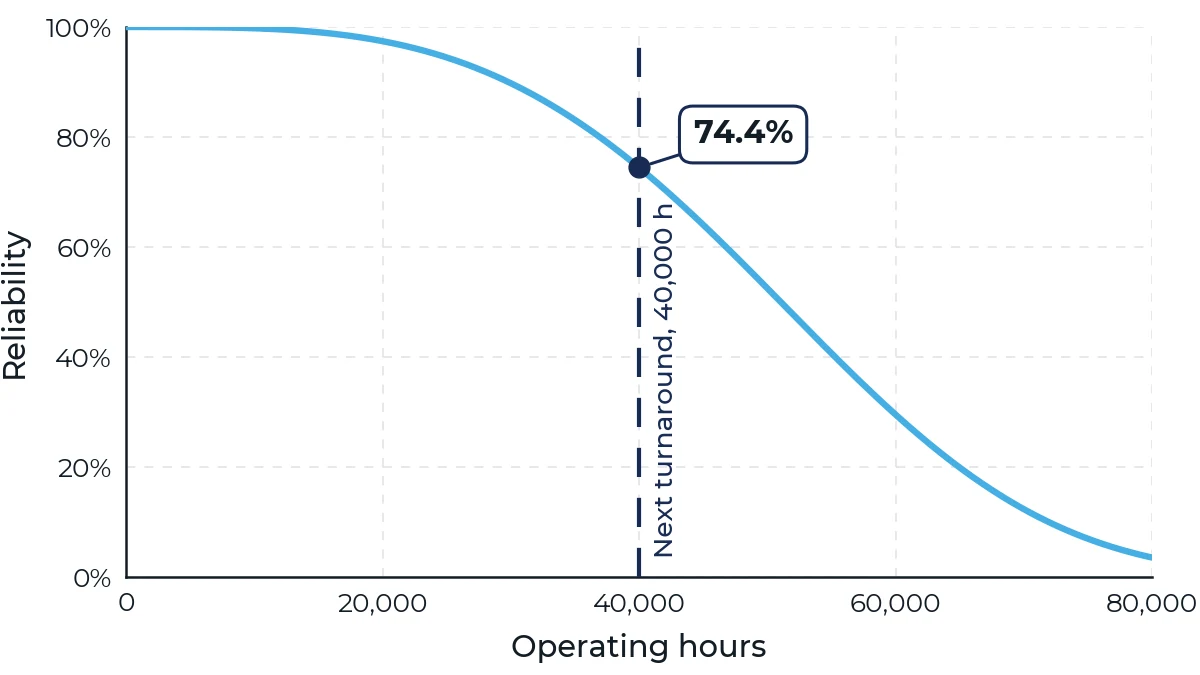
The 90% row is the one worth taking to a shutdown planning meeting, and here is exactly what it says, in plain terms: given the hours these 48 tubes have already run, and given that creep rupture behaves the way this alloy's history suggests it does, you can be 90% confident the characteristic life is at least 56,700 hours. Carried through to the 40,000-hour shutdown, that means roughly 74 tubes out of every 100 like this one would still be running failure-free at that point. That is a specific, defensible answer to give a planner, and it is a genuinely different claim from "the tubes are fine," which is not a number at all.
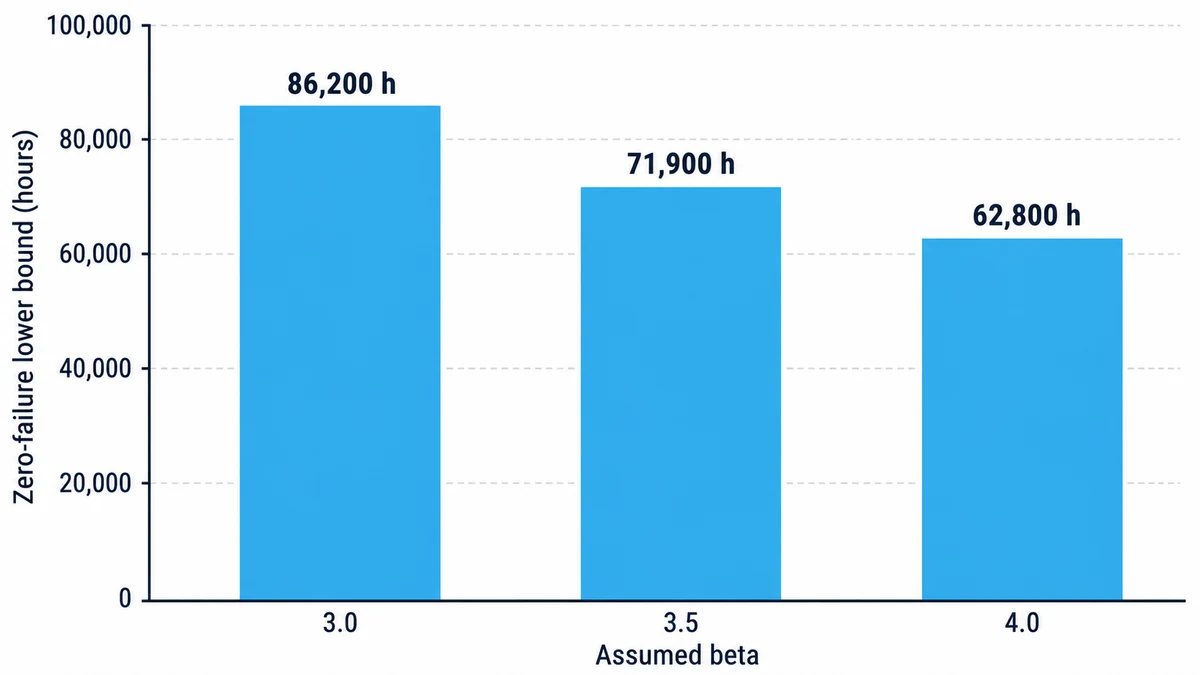
It is also a conditional answer, and the assumed beta is exactly where that condition lives. Holding the same 48 tubes' running hours fixed and only changing the assumed beta shows how much the number moves: at beta 3.0 the bound rises to about 86,200 hours; at beta 4.0 it falls to about 62,800 hours. The direction of that swing matters more than its size. A steeper true mechanism than assumed means the real bound was smaller than reported, an overstatement that creates false confidence, the dangerous direction to be wrong in. A gentler true mechanism than assumed means the real bound was larger than reported, a costly but safe direction, since it only means the fleet was underrated. Stating the assumed beta alongside the bound, every time, lets whoever reads the number see which of those two risks they are exposed to.
None of this proves the new alloy has solved the creep problem for good, and it should not be reported that way. A component with zero observed failures may genuinely be performing well, may simply not have run long enough yet to reveal a problem, or may be developing a different failure mechanism the assumed beta never accounted for. Nothing in the arithmetic above can tell those three apart. Only inspection, condition monitoring, or more running time can, and a Weibayes bound is meant to sit alongside that evidence, not replace it.
Proving a Target Before It Is Installed: Substantiation Testing
Everything so far starts from hours a fleet has already accumulated in the field. Sometimes the question runs the other way: nothing has been installed yet, and you need to prove, on purpose, that a target life is achievable before committing to a purchase, a warranty argument, or a design change across every unit on site. That is substantiation testing, and it uses the same formula, solved for a different unknown.
- t
- the required test duration for every unit on test
- eta sub g
- the characteristic life target the test is meant to demonstrate
- alpha
- one minus the confidence level the demonstration must reach
- N
- the number of units on test, run in parallel for the same duration
- beta
- the assumed shape parameter, exactly as above
This is the lower-bound formula rearranged to solve for the test duration a target demands, instead of the bound a fixed exposure supports, with zero failures allowed anywhere in the test (Abernethy 2006). Suppose the refinery wanted to formally demonstrate a 100,000-hour target for these tubes at 90% confidence, using all 48 as the test population. At the same assumed beta of 3.5, that calculation asks for roughly 42,000 hours of clean running on every one of the 48 tubes, before the target could be called demonstrated.
| Assumed beta | Required hours per tube |
|---|---|
| 3.0 | 36,300 h |
| 3.5 | 42,000 h |
| 4.0 | 46,800 h |
Worth saying plainly: the 48 tubes have only accumulated about 1,124,000 combined running hours so far, against a combined total of roughly 2,015,000 hours a full 90% demonstration at beta 3.5 would require, or a little over half. Run the same numbers forward instead of backward and that accumulated exposure currently supports about 27% confidence in the 100,000-hour target, not 90%. Neither figure is a disappointment. Both are simply what the fleet's actual running time can honestly support today, stated plainly rather than assumed away.
Where This Actually Gets Used

Four situations bring engineers to this method more often than any other. Accepting new equipment against a design life, when commissioning has only produced a handful of running hours so far. Validating a design change, exactly the retube scenario worked through above, where a modification is expected to extend eta without changing the mechanism that sets beta. Checking a vendor's stated life claim against what your own site's running hours actually support, in either direction. And building the case for stocking a critical spare when the failure history is thin by nature: the cost of holding one unbudgeted spare against a defensible lower bound is a far smaller number to defend on a capital plan than an unplanned outage with no spare on the shelf and no defensible reason for having assumed one was not needed.
The Takeaway
A clean run history is not empty of information. It is data that ordinary Weibull fitting cannot use on its own, and treating it as unusable wastes exactly the evidence a thin fleet has actually earned. Weibayes converts running hours into a stated, appropriately narrow claim: not that the design is reliable, but that its characteristic life is at least this much, at this confidence, given this stated assumption about how its risk grows with age. That is a smaller claim than "it's fine," and it is the one you can actually defend in a shutdown meeting.
The next page in this series moves from single components to systems, building reliability block diagrams from the same kind of defensible component-level figures this page, and the four before it, have shown how to produce.
If a critical asset on your site has run clean for years and you need a defensible number rather than a comfortable feeling about it, we would be glad to work through the analysis with you.
Start the conversation