
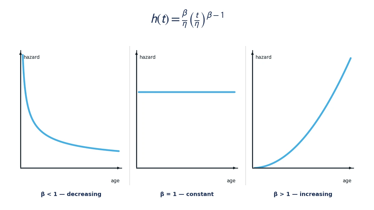
A Weibull distribution is not a curve you fit because the software offers it. It is a direct consequence of one design decision: build a hazard function h(t) that can take almost any monotonic shape, decreasing, flat or increasing, from a single, three-parameter form. That one design decision is why a Weibull can describe a batch of bearings failing early from a bad grease charge, a fleet of relays failing at random from voltage transients, and a set of gearboxes wearing out on schedule, all with the same underlying mathematics and none of the awkward compromises a single fixed-shape distribution would force.
This page builds the Weibull distribution from that idea rather than presenting its formula as something to memorise. Every parameter earns its place here for a physical reason: β selects the shape of the hazard, η fixes the scale of the population's life, and γ, when it belongs at all, shifts the whole clock to account for a genuine failure-free period. Get comfortable with what each one is actually doing, and every plot, every fitted line and every replacement-interval decision later in this series stops being a procedure and starts being something you can reason about directly.
Two facts carry more weight than any other on this page, because a working reliability engineer reaches for them daily: β tells you the character of the failure mechanism at work, and η is always the age by which 63.2% of the population has failed, no matter what β is. Everything else below either builds toward those two facts or extends them.
Building Weibull From What It Has to Explain
A distribution family earns its place in reliability engineering by how well its hazard function h(t) can match the physical mechanisms engineers actually observe. Some mechanisms produce a hazard that falls with age. Others produce a hazard that stays flat. Others produce a hazard that climbs. A distribution that can only represent one of those shapes forces every failure mode into an assumption it may not deserve.
The Weibull distribution's defining trick is a hazard function with exactly one shape-controlling exponent, and that exponent alone is enough to sweep across all three behaviours. Decreasing, constant and increasing hazard are not three different distributions in the Weibull family; they are three settings of the same parameter. That is the entire reason one distribution family covers so much ground in applied reliability work, and it is worth holding onto as the organising idea for everything that follows.
The Weibull Functions, Two Parameters and Three
The two-parameter Weibull describes a population whose risk begins accumulating from age zero. Every quantity below is built from the same two numbers, β and η.
- F of t
- the cumulative distribution function, the fraction of the population failed by age t
- R of t
- the reliability function, the fraction of the population surviving beyond age t
- f of t
- the probability density function, the instantaneous failure rate measured against the original population
- h of t
- the hazard rate, the instantaneous failure rate measured against the population still surviving at t
- beta
- the shape parameter, dimensionless, always positive
- eta
- the scale parameter, the characteristic life, in the same units as t
- t
- age, on the declared time base
These four functions are not four separate ideas bolted together. F(t) and R(t) are complements of the same probability. f(t) is the derivative of F(t). h(t) is f(t) divided by R(t), the conditional version of the same failure behaviour (MIL-HDBK-338B 1998; Abernethy 2006). Notice that the hazard function reduces to a single power law,beta over eta, times t over eta, to the power beta minus one, with no exponential term at all. That simplicity is what makes β so easy to read directly off a hazard curve or a probability plot: it is the exponent, and nothing else in the expression competes with it for shape.
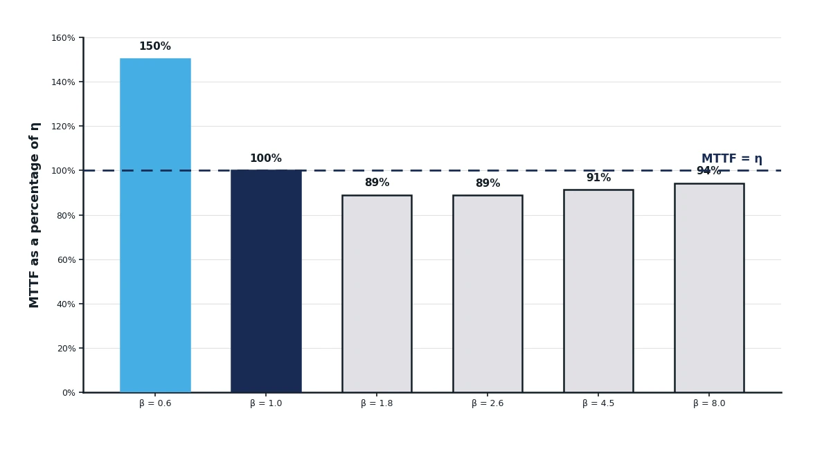
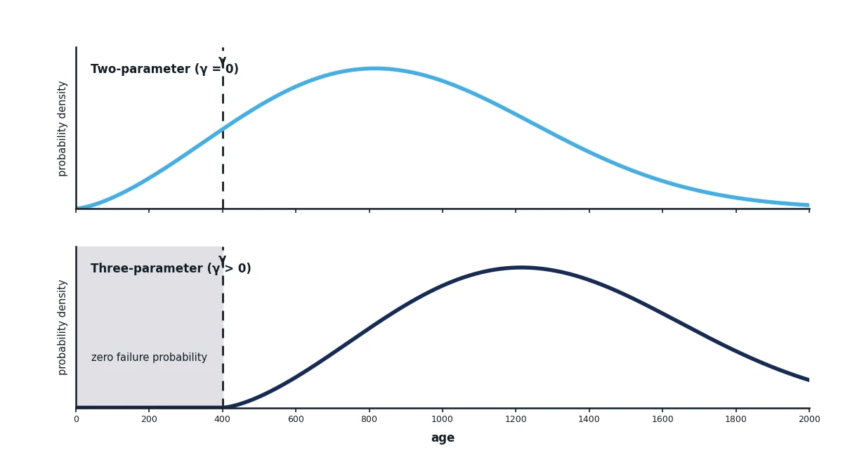
Some populations do not start accumulating risk at age zero. A component with genuine design margin, or a coating with a guaranteed minimum life, can carry a period at the start of its life where failure probability is exactly zero. The three-parameter Weibull adds a location parameter to describe that.
- gamma
- the location parameter, the age below which failure probability from the target mode is exactly zero
Every quantity in the two-parameter form still applies below γ's shift; η is simply measured from γ forward rather than from zero (Abernethy 2006).
Beta Is the Shape: What Each Band Means Physically
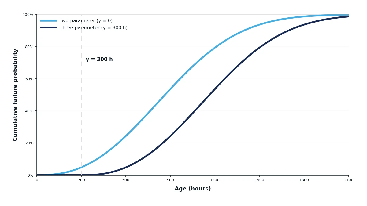
β is the single most informative number in a Weibull analysis, because it is a direct statement about the physical mechanism driving failure, not just a curve-fitting parameter. Reading β correctly tells you what kind of problem you are looking at before you have inspected a single failed unit.
Five bands cover the physical cases a reliability engineer meets in practice, each with a distinct mechanism behind it (Abernethy 2006).
| β range | Hazard behaviour | Physical mechanism | Illustrative example |
|---|---|---|---|
| β < 1 | Decreasing | Installation, commissioning or manufacturing defects | A batch of new bearings failing early from a contaminated grease charge |
| β ≈ 1 | Constant | Random overload or an exogenous event, unrelated to age | Insulation flashover from a lightning-induced voltage transient |
| 1 < β < 3 | Increasing, early wear-out | An emerging fatigue or wear mechanism, not yet dominant | Compressor valve plates showing the first stages of fatigue cracking |
| β > 3 | Increasing, rapid wear-out | A dominant, well-defined wear mechanism | Brake friction material approaching its wear limit |
| β very high | Steep, narrow increase | A batch problem, or a single, tightly controlled wear mechanism acting almost uniformly across the fleet | A casting batch sharing one material defect, or a precisely dimensioned seal face wearing almost identically unit to unit |
Two things are worth stating plainly about this table. First, these bands are diagnostic clues, not proof of root cause; a β in the 1 to 3 range is consistent with early wear-out, but confirming which wear mechanism requires physical inspection, not just the number. Second, a low β does not mean a component is unreliable and a high β does not mean it is reliable; β describes the shape of the risk over age, never its overall level. A β of 0.5 with a long η can still describe a population that rarely fails; a β of 6 with a short η can describe one that fails often, right on schedule. Reading β and η together, never one without the other, is the discipline that separates a useful analysis from a misleading one.
Eta Is Always the 63.2% Life
η carries a property that holds for every single value of β, without exception, and it is the fact that makes a Weibull plot readable at a glance.
This result does not depend on β. Substituting t = η always cancels the exponent to 1, so every Weibull population, whatever its shape, has 63.2% of its members failed by age η.
This is worth sitting with, because it is easy to state and easy to underuse. It means that on any Weibull probability plot, regardless of how steep or shallow the fitted line is, η is always found at the same horizontal reference: the age at which the line crosses 63.2% cumulative failure. You do not need to know β to find η on a plot. You find the 63.2% line, read across to the fitted line, and read down to the age. That single fact is the anchor the whole plotting method in the next stage of this series is built on.
η is a genuine scale parameter in the strict mathematical sense: multiplying every age in a data set by a constant multiplies η by the same constant and leaves β completely unchanged. That is a useful sanity check when comparing two Weibull fits reported in different time units, hours against days, for instance, and it is also why η, not β, is the parameter that shifts when duty or utilisation changes across a fleet.
Why the Mean Is Not Eta: MTTF and the Gamma Function
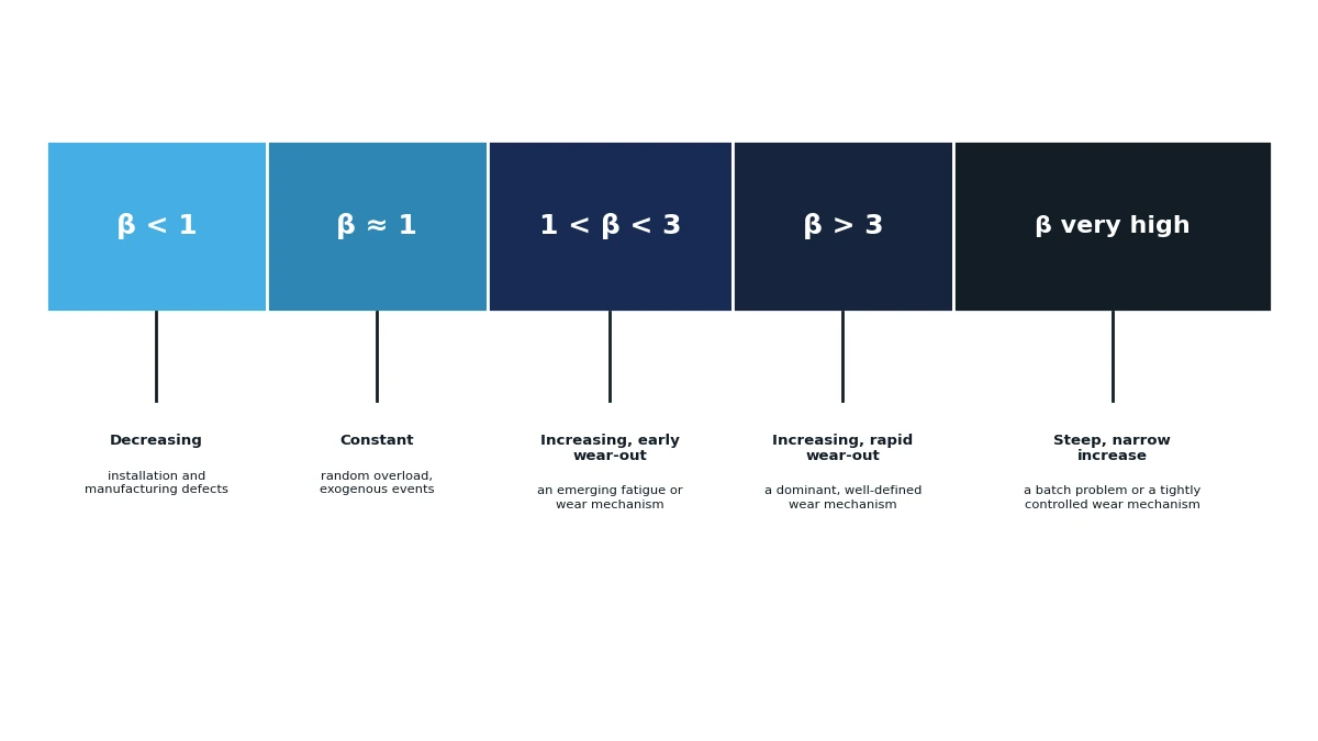
η is often described casually as “the average life,” and that description is wrong often enough, and consequentially enough, to correct directly: η is the 63.2% life, not the mean. The actual mean, the mean time to failure, is a related but distinct quantity.
- MTTF
- the mean time to failure, the arithmetic average life of the population
- gamma of x
- the gamma function, the continuous extension of the factorial to non-integer arguments
Γ(1 + 1/β) is a smooth, well-tabulated function of β alone, and it is worth seeing what it does across the same bands introduced above (Rinne 2009).
| β | Γ(1 + 1/β) | MTTF as a fraction of η |
|---|---|---|
| 0.6 | 1.5046 | MTTF is 50% above η |
| 1.0 | 1.0000 | MTTF equals η exactly |
| 1.8 | 0.8893 | MTTF is 11% below η |
| 2.6 | 0.8882 | MTTF is 11% below η |
| 4.5 | 0.9126 | MTTF is 9% below η |
| 8.0 | 0.9417 | MTTF is 6% below η |
Read this table as a single continuous statement rather than six isolated numbers. For β below 1, the mean sits above η, because a decreasing hazard leaves a long tail of survivors that pulls the average upward. At β = 1 the two are identical. For every β above 1 the mean sits below η, reaching its lowest fraction of η somewhere in the early-wear-out band before climbing back toward η as β grows very large and the distribution narrows around its characteristic life. MTTF < η whenever β > 1, and that gap is exactly why quoting η as “the average life” understates the population's real mean life in the one region, increasing hazard, where the distinction is most likely to affect a decision.
The Exponential Distribution Is Simply Weibull at β = 1
One special case of this relationship deserves its own moment, because it is the cleanest possible way to see how the exponential distribution fits inside the Weibull family rather than standing apart from it. At β = 1, Γ(1 + 1/1) = Γ(2) = 1 exactly, so MTTF = η with no gap at all. The Weibull hazard beta over eta, times t over eta, to the power beta minus one collapses to a flat constant 1/η, and the whole distribution reduces to the familiar exponential form. Every property of the exponential distribution is a direct, unremarkable consequence of setting β to exactly 1 in the machinery already on this page; there is no separate theory to learn.
A worked example makes the general relationship concrete.Take a fleet of compressor valve plates in continuous service, all monitoring one failure mode, fatigue cracking at the seat contact, on operating hours as the time base. Suppose analysis of the fleet's life data (the method for getting from raw ages to a fitted line is the subject of the next page in this series) returns β = 2.6 and η = 18,000 hours.
| Quantity | Formula | Value |
|---|---|---|
| Characteristic life (B63.2) | eta | 18,000 h |
| Mean time to failure | eta times gamma of one plus one over two point six | 15,988 h |
| Median life | eta times the natural log of two, to the power one over beta | 15,633 h |
| Most likely single failure age (mode) | eta times one minus one over beta, to the power one over beta | 14,934 h |
| B10 life (10% of the population failed) | eta times minus the natural log of nought point nine zero, to the power one over beta | 7,575 h |
All five figures describe the same population from different angles, and none of them is interchangeable with any other. The characteristic life is 2,012 hours above the mean, a direct consequence of β sitting in the early-wear-out band above 1. A maintenance planner who quoted 18,000 hours as “the average valve plate life” would be overstating the fleet's real mean life by roughly 13%, small enough to go unnoticed in a single decision and large enough to compound across a portfolio of similar calls.
Gamma: The Location Parameter, and the Discipline It Demands
A positive γ makes a specific physical claim: this population genuinely cannot fail from the target mode before age γ. That is a strong claim, and it needs to be earned by the mechanism, never adopted simply because it makes a plotted line straighter.
The physical cases where a positive γ is legitimate are narrow and specific: a coating or lining with a guaranteed minimum wear allowance before the failure mechanism can begin at all, a component with a design margin that must be consumed before a fatigue crack can initiate, or a coating system with a certified minimum service period. In each case, γ is not a fitted convenience; it is a number an engineer could defend from the design basis independently of any life data at all.
Because a third parameter will almost always improve the apparent fit of a curve to noisy data, whether or not a genuine threshold exists, the decision to include γ needs its own discipline rather than a fit-quality trigger alone (Abernethy 2006):
- Confirm the curvature is systematic, not the result of one or two points. A single early or late failure can bend a plotted line on its own; γ should never be fitted to accommodate an outlier that a separate data-quality review would otherwise flag.
- Require a physical explanation that exists independently of the data. A design margin, a certified coating thickness or a known burn-in specification justifies γ. “The line looks straighter this way” does not.
- Check that γ stays below every observed failure age. A fitted γ that exceeds the youngest recorded failure is not describing a failure-free period; it is describing a mathematical artefact, and the model should be rejected on that basis alone.
- Confirm the improvement is meaningful, not marginal. A location shift that improves a fit statistic by a fraction of a percent rarely justifies the extra parameter and the extra uncertainty that comes with estimating it from the same, usually limited, data set.
Skipping this discipline is exactly how a three-parameter Weibull earns its reputation as “the model that always fits better”: with one more free parameter, it very often will, on data that carries no failure-free period at all. A fit statistic can only tell you how well a line matches points already on the page. It cannot tell you whether γ describes something physically real, and treating a better fit as sufficient justification on its own is the misconception this discipline exists to prevent.
When Weibull Is Not the Right Choice
Weibull's flexibility is wide, not infinite, and forcing it onto data that belongs to a different family produces the same problem a mismatched hazard assumption always produces: a plausible-looking answer that describes the wrong mechanism.
Repair times, and failure mechanisms driven by multiplicative or proportional degradation such as crack growth or diffusion-controlled processes, are usually better described by a lognormal distribution, whose right-skewed shape matches how these durations actually cluster: many short values, a long tail of occasional very long ones. A wear mechanism that is tightly controlled around a single, well-defined mean, with genuinely symmetric scatter either side of it, is sometimes better described by a normal distribution instead.
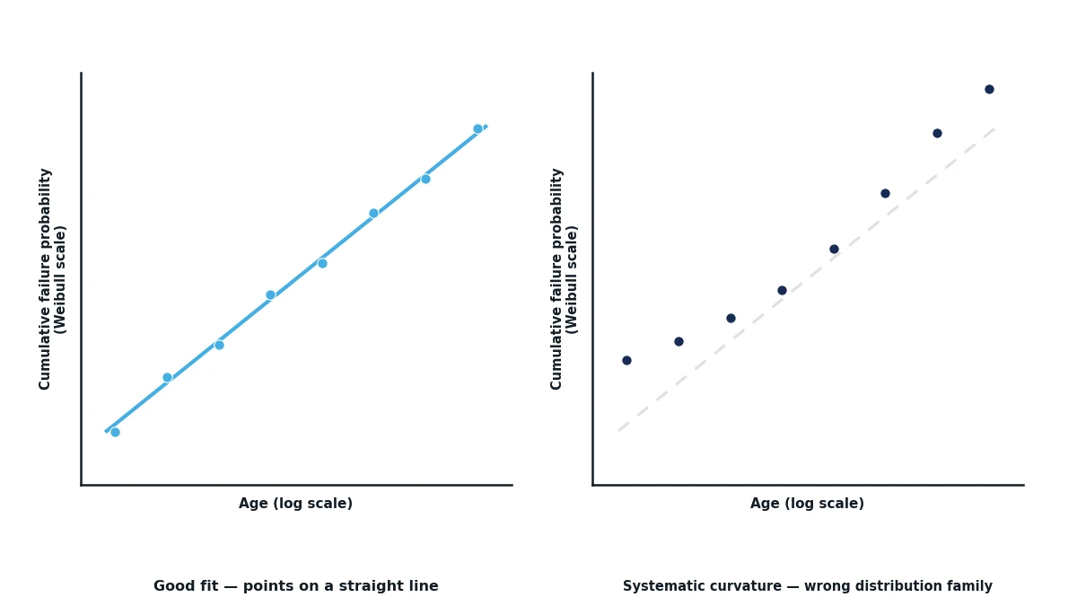
The good news is that a practitioner rarely has to choose blind. The plot itself signals the mismatch: data from a genuinely Weibull-distributed population falls close to a straight line on Weibull-transformed axes, and systematic curvature, rather than the ordinary scatter of a small sample, is the plot telling you the wrong distribution family is in play (Abernethy 2006). Reading that signal correctly, and knowing what a corner or a bend in the line means as distinct from a smooth curve, is a full topic on its own and is where this series goes next.
One Family, Selected by Its Shape
Every idea on this page traces back to the same starting point: a hazard function with one shape-controlling exponent, flexible enough to describe a falling risk, a flat risk or a rising risk from the same three-parameter form. β tells you which of those three behaviours you are looking at, and does so with enough physical specificity to point toward a mechanism before an inspection confirms it. η is always the 63.2% life, a fixed reference point that holds regardless of shape, which is exactly what makes a Weibull plot readable at a glance. γ, used sparingly and only when the mechanism earns it, accounts for a genuine failure-free period without becoming an excuse to force a straighter line through data that does not have one.
None of this is a magic curve-fit. It is a family of hazard shapes, precisely parameterised, and reading β, η and γ correctly is what turns a fitted line into an engineering statement you can defend.
If your team is looking at a fitted β and η and wants a second opinion on what the shape is actually telling you about the failure mechanism, or whether a three-parameter fit is earning its extra complexity, we would be glad to talk it through.
Start the conversation