
In brief
- A capital request that compares two options on purchase price alone has already answered the wrong question: acquisition cost is the smallest and least revealing number in an asset's financial life.
- Lifecycle costing puts the total cost of owning and operating an asset across its useful life on the table before the capital is committed, drawing on the same maintenance history, condition data, failure frequency and operating cost a sound reliability programme depends on.
- Two options with identical total spend can produce very different lifecycle costs, because when the money moves matters as much as how much moves: Net Present Value and Equivalent Annual Cost put competing spending patterns on one comparable basis.
- Every asset has an economic life, the age at which the annual cost of keeping it running starts to exceed the annual cost of replacing it, and that age, not a depreciation schedule, is what should set the renewal decision.
- The lifecycle cost models that survive a capital committee's questions share three characteristics: documented assumptions, sensitivity testing and traceable data provenance.
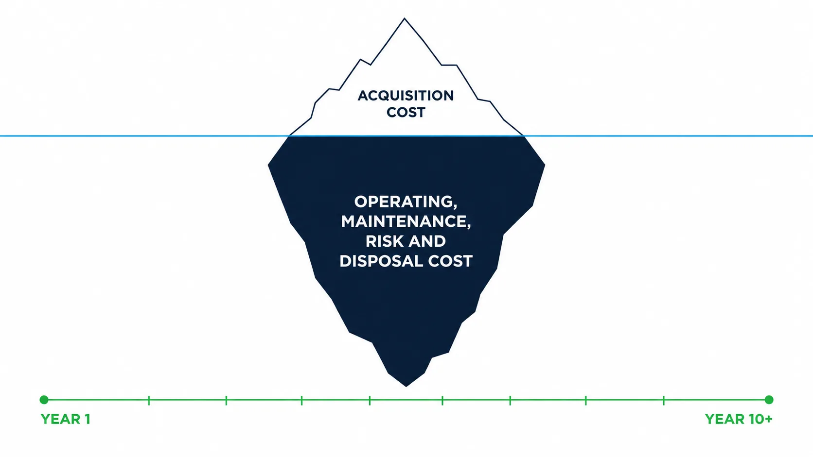
A capital request that compares two options on purchase price alone has already answered the wrong question. Acquisition cost is the smallest and least revealing number in an asset's financial life, yet it is the number most business cases lead with and the number a committee remembers longest. Asset lifecycle costing exists to correct that. It puts the total cost of owning and operating an asset across its useful life on the table before the capital is committed, not after the maintenance bills start arriving.
Lifecycle costing is not a finance exercise bolted onto an engineering decision after the fact. It draws on maintenance history, condition data, failure frequency and operating cost, the same inputs a sound reliability programme depends on, and converts them into the financial language a capital committee uses to approve or reject an investment. Done well, it changes which options survive the shortlist. Done poorly, the asset that looked cheapest on the purchase order quietly becomes the most expensive asset in the fleet to own.
This article sets out what a lifecycle cost model actually calculates, the data it depends on, how the time value of money changes the comparison between competing options, how to find the point at which replacing an asset becomes cheaper than continuing to keep it, and what separates a model that survives a capital committee's questions from one that gets sent back for rework.
What Lifecycle Costing Actually Calculates
Lifecycle costing answers a question acquisition price cannot: what will this asset cost across every year you intend to own it, not just the year you buy it.
The starting point is Total Expenditure, or TOTEX, the combination of Capital Expenditure (CAPEX, spent on acquisition, construction, major overhauls and upgrades) and Operating Expenditure (OPEX, spent on routine maintenance, spares, labour and consumables) across an asset's full life. TOTEX matters because CAPEX and OPEX pull against each other. A lower acquisition price frequently means a lighter-duty design, cheaper materials or reduced redundancy, and those choices show up later as higher operating and maintenance spend. A model that only tracks CAPEX, or only tracks OPEX, will always be blind to that trade-off.
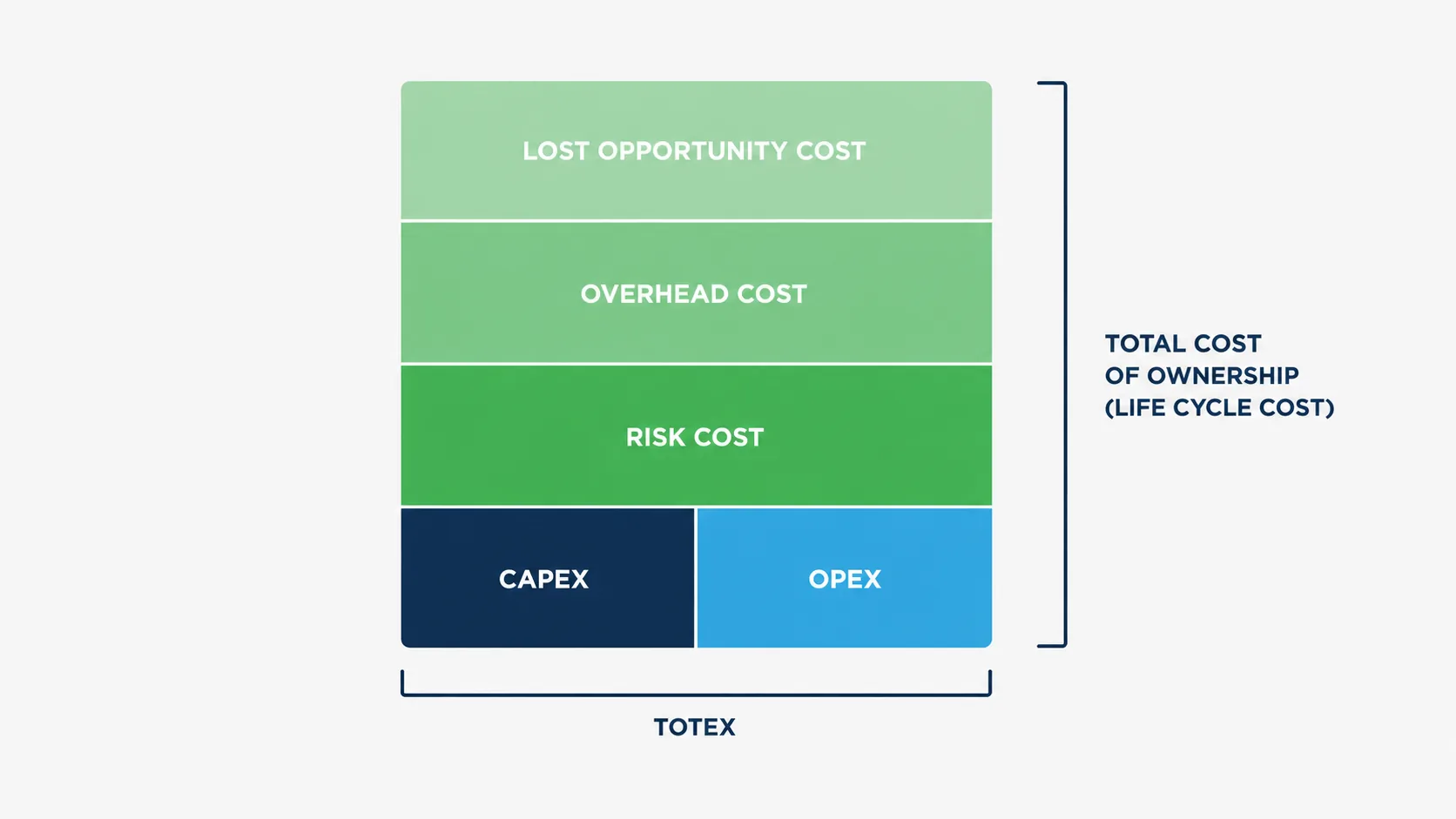
The figure asset managers actually work with is the Total Cost of Ownership, sometimes called Life Cycle Cost. This is TOTEX with three further additions: the risk cost of things that might go wrong, the overhead cost of the systems and people needed to support the asset through its life, and the lost opportunity cost of any performance limitation or downtime the asset causes. A lifecycle cost model that stops at capital and maintenance spend and ignores these three additions will consistently understate the true cost of the cheaper-looking option, because reliability risk and lost production rarely show up as a line item until they have already happened.
A useful way to see the scope of a lifecycle cost model is the activities it has to cost: acquisition and installation, operation, maintenance, the support services that keep all of the above running, and disposal. Leave any one of these off the model and the comparison between options is no longer a fair one.
The Inputs a Defensible Model Cannot Do Without
A lifecycle cost model is only as credible as the data behind it, and that data comes from four places: maintenance history, condition data, failure frequency and operating cost.
Maintenance history is the record of what has actually been spent keeping the asset running, labour, parts and contractor costs, and is the foundation for projecting future operating and maintenance spend. Condition data, from inspection results or continuous condition monitoring, tells you where the asset actually sits on its degradation curve, rather than where a generic assumption places it. Failure frequency, the kind of data a properly conducted FMECA or RCM study produces, lets the model reflect how this specific asset actually fails rather than an industry rule of thumb. Operating cost, energy and consumables tied to throughput, completes the picture.
These four inputs are what let a lifecycle cost model describe the asset in front of you instead of a generic version of it. A model built without them can still produce a number, but the number reflects the quality of the assumptions behind it rather than the condition of the asset, which is exactly what a capital committee is testing when it asks where the figures came from. Well-structured, consistently coded maintenance and condition records make this part of the model fast to build and hard to argue with.
Why the Timing of Money Changes the Answer
Two options with identical total spend across their working life can produce very different lifecycle costs, because when the money moves matters as much as how much moves.
This is the time value of money: a dollar spent or saved in year one is worth more than a dollar spent or saved in year ten, because money available today can earn a return between now and then. Net Present Value (NPV), the total present value of a series of future cash flows discounted back to today at the organisation's cost of capital, is the tool that puts every option's spending pattern onto a common, comparable basis. Equivalent Annual Cost (EAC) takes that NPV and converts it into a regular annual amount, useful for comparing options with different lives, or for comparing a purchase against a lease.
Illustrative example
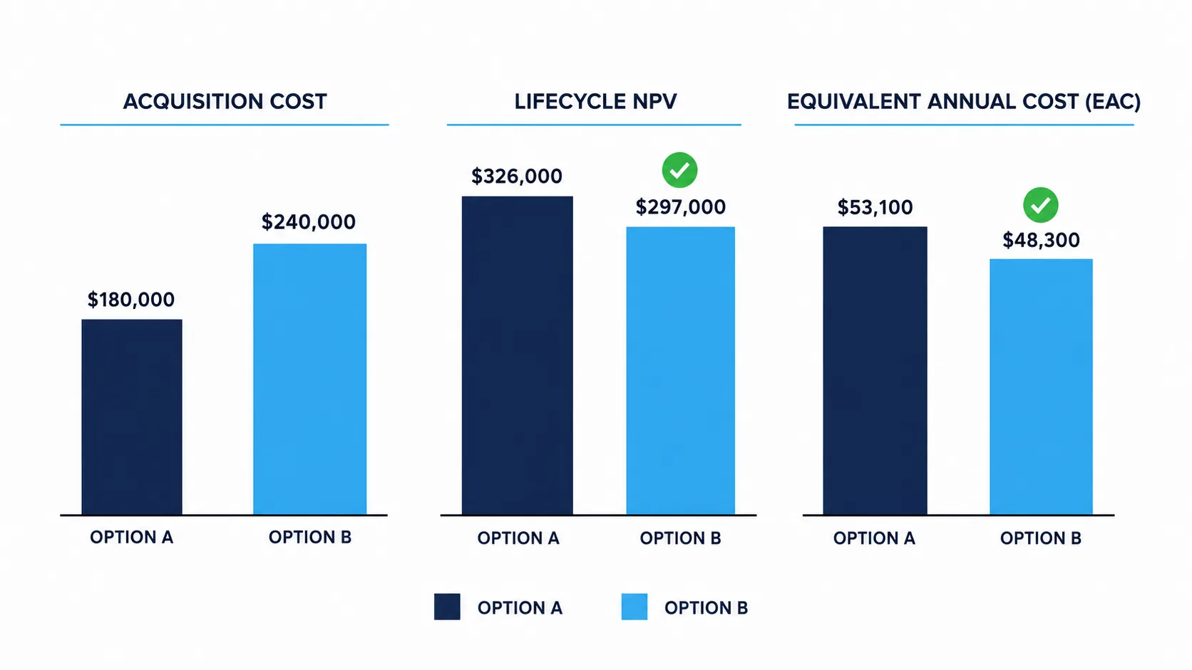
Consider two options for a critical piece of rotating equipment, each with a ten-year working life and a 10 per cent discount rate. Option A costs $180,000 to acquire, and its operating and maintenance cost starts at $18,000 in year one and climbs by roughly 8 per cent a year as wear accelerates, offset by a modest disposal credit in year ten. Option B costs $240,000 to acquire, a $60,000 premium reflecting better metallurgy and a more reliable design, and its operating and maintenance cost starts lower at $9,000 and climbs by only around 4 per cent a year, with a larger disposal credit at the end of its life.
Discounted at 10 per cent, Option A's lifecycle cost has an NPV of approximately $326,000 and an EAC of approximately $53,100 a year. Option B's lifecycle cost has an NPV of approximately $297,000 and an EAC of approximately $48,300 a year. Option A is $60,000 cheaper to buy. Option B is roughly $29,500 cheaper across its lifecycle in present value terms, and roughly $4,800 a year cheaper on an equivalent annual cost basis. Acquisition price and lifecycle cost produce two different winners, which is precisely the situation lifecycle costing exists to catch before the capital is committed rather than after.
Finding the Economic Life: When Keeping an Asset Costs More Than Replacing It
Every asset has an age at which the annual cost of keeping it running starts to exceed the annual cost of replacing it, and that age, not a depreciation schedule, is what should set the renewal decision.
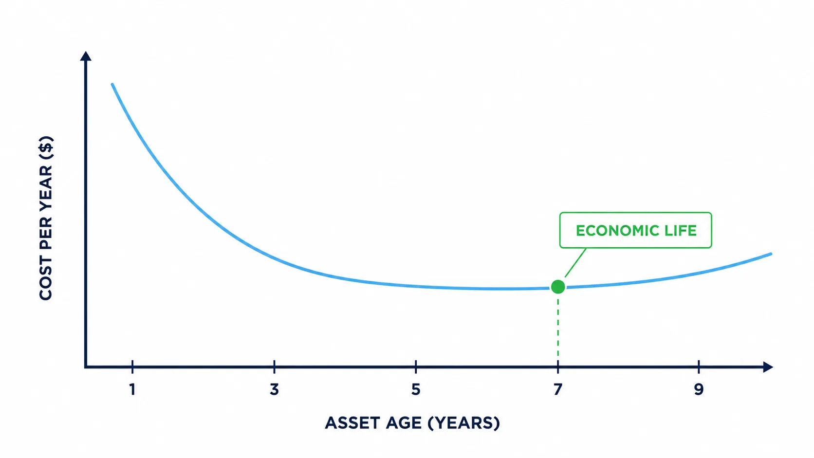
This age is the asset's economic life: the point that minimises the total cost per year of owning it, or, once discounting is applied, the point that minimises its EAC. The mechanic behind it is straightforward. As an asset ages, its acquisition cost gets spread over more years of service, which pulls the average cost per year down. At the same time, operating and maintenance cost typically climbs as wear accumulates, which pushes the average cost per year up. Economic life is the age at which these two effects balance and cost per year is at its lowest, before rising maintenance cost starts to dominate.
Illustrative example
Take an asset acquired for $420,000, with operating and maintenance cost starting at $22,000 in year one and escalating at roughly 30 per cent a year as wear compounds, a realistic pattern approaching the end of a component's service life without intervention. Cost per year falls sharply, from $442,000 at age one to around $139,000 by age four, continues falling to a low of around $115,000 at age seven, then climbs back to around $125,000 by age nine. Age seven is the economic life. Keep the asset beyond that point and average cost starts rising again.
The replacement decision that follows is simple to state: once the annual cost of maintaining an ageing asset exceeds the equivalent annual cost of replacing it, deferring the decision is no longer the cheaper path. It is the path that defers the cost into a future budget, typically at a higher total cost once escalating breakdown risk is included. Real assets rarely escalate on a smooth curve, which is why the condition and failure frequency data covered earlier matters here, letting the escalation curve reflect the specific asset under review rather than a generic assumption.
Judging the Investment: The Criteria a Capital Committee Actually Uses
A lifecycle cost model tells you what an option costs. A set of investment criteria tells you whether that cost is good enough to approve.
- Minimum Acceptable Rate of Return (MARR), or hurdle rate: the minimum return an organisation requires from a capital investment before it approves funding, typically 15 per cent or higher in industrial organisations, built up from the cost of capital, a margin for risk and an expectation of profit.
- Internal Rate of Return (IRR): the discount rate at which a project's NPV equals zero. It is tested against the hurdle rate to judge whether an investment clears the bar the organisation has set.
- Payback period: how quickly the investment is recovered. A shorter payback reduces exposure to the risk that cost or revenue estimates drift over time.
- Profitability Index: the NPV of the returns divided by the investment required. It must exceed 1.0 for a project to be financially viable, and gives a quick way to rank competing proposals of different sizes.
Returning to the pump comparison: the extra $60,000 to select Option B over Option A is itself an investment, and it can be tested the same way. The savings it generates, in lower operating cost and a larger disposal credit, produce an IRR of approximately 18 per cent on that incremental spend. Against a 15 per cent hurdle rate, that clears the bar, and on an undiscounted basis it pays back within roughly six years. The lifecycle model shows Option B costs less to own. The investment criteria confirm the extra $60,000 upfront is, on its own terms, a financially sound use of capital, not simply a preference for a lower number.
These criteria matter more, not less, as the acquisition premium grows. A capital committee asked to approve a larger cheque wants the return on that spend quantified in the same terms it uses to judge every other investment, not asserted as self-evidently worthwhile.
What Makes a Lifecycle Cost Model Hold Up to Scrutiny
The lifecycle cost models that survive a capital committee's questions share three characteristics, and a model missing even one of them typically gets sent back for rework.
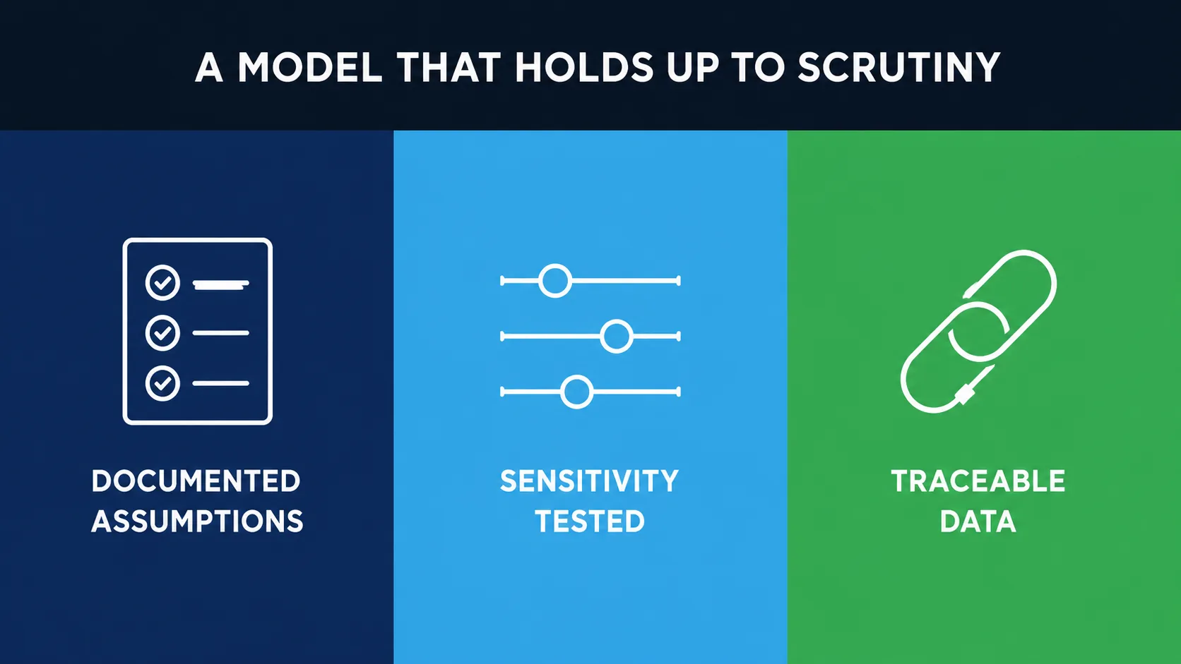
- Documented assumptions. Every discount rate, escalation rate and residual value in the model should be stated explicitly, along with where it came from, rather than buried inside a formula only the person who built the spreadsheet can decode.
- Sensitivity testing. A model that shows how the recommendation changes if the discount rate, escalation rate or assumed useful life moves within a reasonable range demonstrates the conclusion is not fragile to one debatable number, usually the first thing a sharp question in a capital committee meeting will probe.
- Traceable data provenance. The maintenance history, condition data and failure frequency behind the model need to be traceable back to source records, not summarised as based on experience, because a number that cannot be traced cannot be defended when it is challenged.
This is where the financial and non-financial sides of asset management need to work from the same picture, not as two separate exercises that happen to arrive at the same report. ISO 55001 already points this way, requiring that the financial and non-financial implications of managing assets over their life cycles be determined and documented. ISO/TS 55010, the technical specification giving guidance on aligning financial and non-financial asset management functions, exists because the numbers finance reports and the condition and risk data engineering holds need to describe the same assets consistently if either is to be trusted. A model built on that alignment is not just more accurate. It is defensible in a way one built in isolation from either side never quite manages to be.
Building Lifecycle Costing Into the Asset Management System
Lifecycle costing pays off when it is built into the system, not reconstructed from scratch for every capital request.
A Strategic Asset Management Plan sets the direction, an Asset Management Plan translates it into managed activities, and criticality determines where a full lifecycle cost model is justified against a lighter assessment. Lifecycle cost models belong inside that governance structure as living documents, refreshed as new condition and failure data arrives, not one-off calculations filed away once capital is approved. The model built for one renewal decision becomes the baseline for the next, and forecasting sharpens with every cycle as outcomes are compared against the assumptions documented at the time.
At a portfolio level, this discipline rolls up into the benchmark a board reviews: maintenance cost as a percentage of Replacement Asset Value, typically 2 to 4 per cent for well-managed continuous process assets and 4 to 7 per cent for heavy industrial assets. Individual lifecycle cost decisions, made well and consistently, are what keep that portfolio-level number defensible rather than aspirational.
The Decision the Model Is Actually Making
Every capital request eventually reduces to a single comparison: what does it cost to keep what you have, against what does it cost to replace it, expressed in the same currency and on the same time basis. Acquisition price alone cannot answer that question, and neither can accumulated maintenance spend on its own. A lifecycle cost model built on real condition and failure data, discounted properly, tested against a hurdle rate the organisation actually uses, and documented well enough to survive being questioned, turns that comparison from a negotiation into an evaluation.
That is the difference between a business case approved because nobody in the room could find the flaw in it, and one approved because there genuinely wasn't one.
Frequently asked questions
What is asset lifecycle costing?
Asset lifecycle costing puts the total cost of owning and operating an asset across its useful life on the table before the capital is committed, not after the maintenance bills start arriving. It covers acquisition and installation, operation, maintenance, the support services that keep all of the above running, and disposal.
What is the difference between TOTEX and Total Cost of Ownership?
TOTEX, or Total Expenditure, is the combination of Capital Expenditure (CAPEX, spent on acquisition, construction, major overhauls and upgrades) and Operating Expenditure (OPEX, spent on routine maintenance, spares, labour and consumables) across an asset's full life. Total Cost of Ownership, sometimes called Life Cycle Cost, is TOTEX with three further additions: the risk cost of things that might go wrong, the overhead cost of the systems and people needed to support the asset, and the lost opportunity cost of any performance limitation or downtime the asset causes.
What is the economic life of an asset?
The economic life of an asset is the age at which the annual cost of keeping it running starts to exceed the annual cost of replacing it: the point that minimises the total cost per year of owning it, or, once discounting is applied, the point that minimises its Equivalent Annual Cost.
What is Equivalent Annual Cost (EAC)?
Equivalent Annual Cost takes an asset's Net Present Value and converts it into a regular annual amount, which is useful for comparing options with different working lives, or for comparing a purchase against a lease.
What is the Minimum Acceptable Rate of Return (MARR) for a capital investment?
The Minimum Acceptable Rate of Return, or hurdle rate, is the minimum return an organisation requires from a capital investment before it approves funding, typically 15 per cent or higher in industrial organisations, built up from the cost of capital, a margin for risk and an expectation of profit.